Understanding conventional HMM-based ASR training
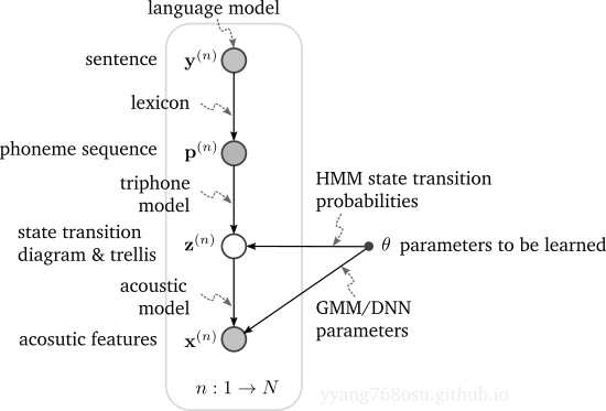
Conventional HMM-based ASR system assumes a generative model comprised of a language model, a lexicon (e.g., pronunciation dictionary), and an acoustic model, as illustrated below. Here \(\theta\) denotes the parameters to be learned and it comprises of the HMM state transition probabilities and GMM/DNN parameters.
Maximum likelihood training
In maximum likelihood estimation (MLE), as stated in the equation below, the objective is to maximize the likelihood of the data being generated by the generative model. In other words, we want to find the value of the parameters \(\theta\) so that the above model best explains the acoustic features (e.g., spectrogram) that we observe.
\[\begin{align*} &\arg\max_\theta \prod_{n=1}^N \mathbb{P}\left({\bf x}^{(n)}|{\bf y}^{(n)};\theta\right)\\ =&\arg\max_\theta \sum_{n=1}^N \log \mathbb{P}\left({\bf x}^{(n)}|{\bf y}^{(n)};\theta\right). \end{align*}\]For ease of notation, for the rest of this section, let’s ignore the conditioning on \({\bf y}^{(n)}\) (or \({\bf p}^{(n)}\)). The difficulty in evaluating the above log-likelihood lies in the need to marginalize over all potential values of \({\bf z}^{(n)}\). This formulation falls right into the discussion of the previous two posts: variational lower bound and expectation maximization, which provide an iterative algorithm to approach the solution
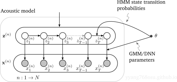
\[\begin{align} \theta^{[i+1]} = \arg\max_{\theta} \sum_{n=1}^N \int \color{red}{\mathbb{P}\left({\bf z}^{(n)}| {\bf x}^{(n)};\theta^{[i]} \right)}\log \mathbb{P}\left({\bf x}^{(n)}, {\bf z}^{(n)};\theta\right)d z^{(n)}. \end{align}\]Most of the computation complexity in the above equation lies in finding the posterior probability of the latent state given the observed \(\color{red}{\mathbb{P}\left({\bf z}^{(n)}\| {\bf x}^{(n)};\theta\right)}\). To elaborate on how the posterior probability is computed, let’s expand the acoustic model part in the previous figure as below, which is essentially a hidden-Markov chain.
The inference problem (finding the posterior of the latent given the observed) in a hidden Markov chain can be solved by a forward-backward algorithm. The algorithm manifests itself as BCJR algorithm in convolutional code bit-level MAP decoding and Kalman filtering in linear dynamic system.
\[\begin{align} \text{Forward path: }&\text{calculate }\mathbb{P}\left(z_t,{\bf x}_{1\to t};\theta\right)\text{ from }\mathbb{P}\left(z_{t-1},{\bf x}_{1\to t-1};\theta\right) \notag \\ &\mathbb{P}\left(z_t, {\bf x}_{1\to t};\theta\right) = \sum_{z_{t-1}} \mathbb{P}(z_{t}|z_{t-1};\theta)\mathbb{P}(x_{t}|z_{t};\theta)\mathbb{P}\left(z_{t-1},{\bf x}_{1\to t-1};\theta\right) \notag \\ \text{Backward path: }&\text{calculate }\mathbb{P}\left({\bf x}_{t+1\to T}{\big |}z_t;\theta\right)\text{ from }\mathbb{P}\left({\bf x}_{t+2\to T}{\big |}z_{t+1};\theta\right) \notag \\ &\mathbb{P}\left({\bf x}_{t+1\to T}{\big |}z_t;\theta\right) = \sum_{z_{t+1}} \mathbb{P}(z_{t+1}|z_{t};\theta)\mathbb{P}(x_{t+1}|z_{t+1};\theta)\mathbb{P}\left({\bf x}_{t+2\to T}{\big |}z_{t+1};\theta\right) \notag \\ \text{Combined: }&\mathbb{P}\left(z_t, {\bf x}_{1\to T};\theta\right) = \mathbb{P}\left(z_t,{\bf x}_{1\to t};\theta\right)\mathbb{P}\left({\bf x}_{t+1\to T}{\big |}z_t;\theta\right) \notag \\ &\mathbb{P}\left(z_t| {\bf x}_{1\to T};\theta\right) = \mathbb{P}\left(z_t, {\bf x}_{1\to T};\theta\right) / \sum_{z_t}\mathbb{P}\left(z_t, {\bf x}_{1\to T};\theta\right) \end{align}\]Circular dependency between segmentation and recognition
The expectation-maximization formulation for likelihood maximization reveals a fundamental circular dependency between segmentation and recognition.
Here segmentation refers to the alignment of sub-phoneme states of \({\bf y}\) and the acoustic feature observations \({\bf x}\), encoded in the hidden state sequence \({\bf z}\), and recognition refers to the classification of sub-phoneme hidden state sequence \({\bf z}\) for the corresponds acoustic feature observations \({\bf x}\).
The two equations below make the circular dependency precise:
\[\begin{align*} \theta^{[i]} & \underset{\text{ }}{\xrightarrow{\substack{\text{update soft-alignment}\\\text{based on recognition}}}} \mathbb{P}\left({\bf z}^{(n)}| {\bf x}^{(n)};\theta^{[i]} \right)\text{ using Equation (2)}\\ \mathbb{P}\left({\bf z}^{(n)}| {\bf x}^{(n)};\theta^{[i]} \right) & \underset{\text{ }}{\xrightarrow{\substack{\text{update recognition}\\\text{based on soft-alignment}}}} \theta^{[i+1]}\text{ using Equation (1)} \end{align*}\]It is easy to argue that to have an accurate alignment, we need accurate recognition, and to train an accurate recognition, we have to rely on accurate alignment/segmentation.
In a conventional ASR system, to bootstrap the training procedure, we have to start with a dataset that has human curated phoneme boundary/segmentation. Once the system is capacitated with reasonable recognition/inference, it is no longer confined with human aligned dataset and a much larger dataset can be used with just waveform and the corresponding phoneme transcription. Eventually, after the system is able to deliver robust segmentation, we can make hard decision on the alignment, and only focus on improving the recognition performance with potentially a different system that has a much larger capacity, e.g., a DNN replacing the GMM model.
Decoding
In the decoding stage, we try to find the word/sentence with the maximum a posterior (MAP) probability given the observed data
\[\begin{align*} &\arg\max_{\bf y} \mathbb{P}({\bf y}|{\bf x};\theta) \\ =&\arg\max_{\bf y} \mathbb{P}({\bf x},{\bf y};\theta) / \mathbb{P}({\bf x};\theta)\\ \color{red}{=}&\arg\max_{\bf y} \mathbb{P}({\bf x},{\bf y};\theta) \\ =&\arg\max_{\bf y} \underbrace{\mathbb{P}({\bf x}|{\bf p};\theta)}_{\text{acoustic model}}\times\underbrace{\mathbb{P}({\bf p}|{\bf y})}_{\text{lexion}}\times\underbrace{\mathbb{P}({\bf y})}_{\text{language model}} \end{align*}\]The lexicon and language model together construct a state transition diagram, which we unrolled in time to form a decoding trellis. For each transcription hypothesis, a proper MAP decoder would sum across all the paths in the trellis that corresponds to the transcription, which is computationally prohibitive.
One simplification one can make is to find the most probable path by running the Viterbi algorithm. However, even for Viterbi algorithm, the complexity is still too high for practical deployment due to the large state space and potentially large number of time steps.
To further reduce the computation complexity, the conventional system resorts to the beam-search algorithm – basically a breath-first-search algorithm on the trellis that maintain only a limited number of candidates. The beam-search algorithm is often run on a weighted finite state transducer that captures the concatenation of language model and lexicon.
Discrepancy between MLE training and MAP decoding
At first glance into the MAP decoding equation, it may appear that the MLE based training is well-aligned with the decoding process: maximizing the posterior probability of the transcription \({\bf y}\) given the acoustic feature \({\bf x}\) is equivalent to maximizing the likelihood of the observation \({\bf x}\). The argument being that the probability of the observation \(\mathbb{P}(x;\theta)\) is anyway a constant dictated by the natural of people’s speech, not something we can control. But is it true?
\[\begin{align*} &\text{inference time:}\\ &\arg\max_{\bf y} \mathbb{P}({\bf y}|{\bf x};\theta) \\ =&\arg\max_{\bf y} \mathbb{P}({\bf x},{\bf y};\theta) / \mathbb{P}({\bf x};\theta)\\ =&\arg\max_{\bf y} \mathbb{P}({\bf x}|{\bf y};\theta)\mathbb{P}({\bf y}) \end{align*}\]It turns out there is a subtle difference between inference time (MAP decoding) and training time (MLE parameter update) that render the above statement wrong.
\[\begin{align*} &\text{training time:}\\ &\arg\max_{\color{red}{\theta}} \mathbb{P}({\bf y}|{\bf x};\theta) \\ =&\arg\max_{\color{red}{\theta}} \mathbb{P}({\bf x},{\bf y};\theta) / \mathbb{P}({\bf x};\theta)\\ \color{red}{\not=}&\arg\max_{\color{red}{\theta}} \mathbb{P}({\bf x}|{\bf y};\theta)\mathbb{P}({\bf y}) \end{align*}\]As is evident by comparing the above two equations, when we try to update parameter \(\theta\) to maximize directly the posterior probability of the transcription \({\bf y}\) given the acoustic feature \({\bf x}\), we can no longer ignore the term \(\mathbb{P}({\bf x};\theta)\). The key is to realize that we model the speech as a generative model, where the probability of observing a certain acoustic features \({\bf x}\) is not dictated by the nature, but rather the generative model that we assume. By updating the parameter \(\theta\) that best increase the likelihood, we inevitably change \(\mathbb{P}({\bf x};\theta)\) too, and thus there is no guarantee that the posterior probability is increased. \(\mathbb{P}({\bf x};\theta)\) is calculated by marginalizing over all potential transcriptions: \(\mathbb{P}({\bf x};\theta)=\sum_{\bf y}\mathbb{P}({\bf x}\|{\bf y};\theta)\).
To elaborate, in MLE, we try to maximize \(\color{red}{\mathbb{P}({\bf y}\|{\bf x};\theta)}\) with respect to \(\theta\), we may very well also increased the likelihood for competing transcription sequences \(\color{blue}{\mathbb{P}({\bf x}\|{\bf \tilde{y}};\theta)}\), potentially resulting in decreased posterior probability \(\mathbb{P}({\bf y}\|{\bf x};\theta)\).
\[\begin{align*} &\mathbb{P}({\bf y}|{\bf x};\theta) \\ =& \mathbb{P}({\bf x},{\bf y};\theta) / \mathbb{P}({\bf x};\theta)\\ =& \frac{\color{red}{\mathbb{P}({\bf x}|{\bf y};\theta)}\mathbb{P}({\bf y})}{\sum_{\bf \tilde{y}}\color{blue}{\mathbb{P}({\bf x}|{\bf \tilde{y}};\theta)}\mathbb{P}({\bf \tilde{y}})} \end{align*}\]Fundamentally, the misalignment is rooted from the fact that we are using a generative model for discriminative tasks. We end here by noting that several sequence discriminative training methods were proposed for better discrimination in the literature.