An introduction to Kalman filter and particle filter
Kalman filter and particle filter are concepts that are intimidating for new learners due to their involved mathematical description, and are straightforward once you grasp the main idea and get used to Gaussian distributions. The goal of this post is to take a journey to Kalman filter by dissecting its idea and operation into pieces that are easy to absorb, and then assemble them together to give the whole picture. As a last step, we will see that particle filter achieves the same goal for non-Gaussian system resorting to Monte Carlo sampling.
Below let’s walk through three simple problems and their solutions stemming from Gaussian distributions, and then stitching them together to form the problem that Kalman filter tries to solve and present its solution.
A. Conditional Gaussian distribution
Here I assume you have a basic knowledge regarding multivariate Gaussian distributions. A multivariate Gaussian distribution is captured by its mean vector and covariance matrix, often denoted as \(\mu\) and \(\Sigma\). Below let us consider the bivariate Gaussian vector \([z,x]^T\), with the following general notation:
\[\begin{align*} \left[ \begin{array}{c} z\\ x \end{array} \right] \sim \mathcal{N} \left( \left[ \begin{array}{c} \mu_z\\ \mu_x \end{array} \right], \left[\begin{array}{cc} \Sigma_z & \Sigma_{zx} \\ \Sigma_{xz} & \Sigma_{x} \end{array}\right] \right)\notag \end{align*}\]The covariance matrix is formally defined as
\[\begin{align*} \left[\begin{array}{cc} \Sigma_z & \Sigma_{zx} \\ \Sigma_{xz} & \Sigma_{x} \end{array}\right] =& \mathbb{E}\left[ \left[ \begin{array}{c} z-\mu_z\\ x-\mu_x \end{array} \right] \left[ \begin{array}{c} z-\mu_z\\ x-\mu_x \end{array} \right]^T \right]\notag\\ =& \left[ \begin{array}{cc} \mathbb{E}[(z-\mu_z)(z-\mu_z)^T] & \mathbb{E}[(z-\mu_z)(x-\mu_x)^T]\\ \mathbb{E}[(x-\mu_x)(z-\mu_z)^T] & \mathbb{E}[(x-\mu_x)(x-\mu_x)^T] \end{array} \right]\notag. \end{align*}\]The off-diagonal term represents the cross covariance between the two random variables \(x\) and \(z\), which, by checking the definition above, satisfies \(\Sigma_{xz}=\Sigma^T_{zx}\). The larger the cross covariance, the more correlated the two random variables are. For correlated random variables, knowing the value of one would help us in guessing the value of the other. Let us take a look at the figure below for a concrete example.
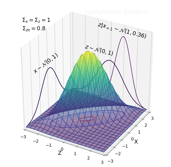
The figure above illustrates the joint distribution of a bivariate Gaussian distribution with \(\mu_z=\mu_x=0\), \(\Sigma_z=\Sigma_x=1\), and \(\Sigma_{zx}=\Sigma_{xz}=0.8\). The marginal distributions of both \(x\) and \(z\) are \(\mathcal{N}(0,1)\). The contour of the distribution forms a thin ellipse, reflecting the strong covariance \(\Sigma_{zx}=\Sigma_{xz}=0.8\) between the two random variables \(x\) and \(z\). To verify that knowing one variable helps estimate the other, let us take a look at the conditional distribution of \(z\) given \(x=1\), and compare it with the marginal distribution of \(z\). As can be seen from the figure above, the distribution of \(z\|x=1\) has much narrower span than \(z\), with a shift in the mean. The reduction of variance of \(z\) after observing \(x=1\) is evidence that the observation of \(x\) narrows down the potential values of \(z\).
An important fact here is that the conditional distribution of a joint-Gaussian distribution is also Gaussian
\[\begin{align*} p(z|x) = p(x,z)/p(x)\sim\mathcal{N}\left(\mu_{z|x}, \Sigma_{z|x}\right)\notag. \end{align*}\]Below are two identities on the general expressions of the conditional distribution, here let us accept them as they are without bothering with any proof.
\[\begin{align*} \mu_{z|x} &= \mu_z + \Sigma_{zx}\Sigma_{xx}^{-1}(x-\mu_x)\notag\\ \Sigma_{z|x} &= \Sigma_{z} - \Sigma_{zx}\Sigma_x^{-1}\Sigma_{xz} \text{ } \left(\preccurlyeq \Sigma_{z}\right) \notag \end{align*}\]The above two equations are very important, and lies in the core of many concepts such as MMSE estimator, Wiener filter and of course, Kalman filter. To see that knowing \(x\) would reduce the uncertainty in \(z\), here let’s just point out that the entropy (measure of uncertainty) of a Gaussian random vector is an increasing function of the determinant of the covariance-matrix, and that \(\Sigma_{z\|x}\) always has a smaller determinant than \(\Sigma_z\) for any non-zero cross covariance \(\Sigma_{zx}\), followed from the second equation with the fact that \(\Sigma_{z}-\Sigma_{z\|x}\) \(=\Sigma_{zx}\Sigma_x^{-1}\Sigma_{xz}\succcurlyeq 0\) is a semi-positive-definite matrix.
These two equations will become useful when we visit part C, and we will come back to them.
B. Gaussian distribution with linear transformation
In the first section we looked at the case of obtaining the conditional distribution from a joint Gaussian distribution, here let’s look at the distribution of a Gaussian vector going through a linear transform. More precisely, let us define a random variable \(z_n\) as obtained from the following transform
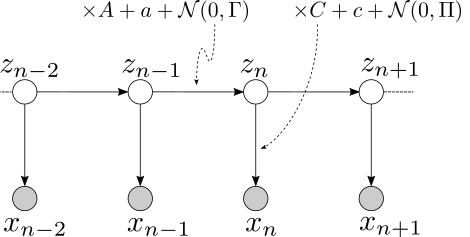
\[\begin{align*} z_{n-1}&\sim\mathbb{N}(\mu_{n-1}, V_{n-1})\notag\\ z_n |z_{n-1}&\sim A z_{n-1}+a+\mathcal{N}(0,\Gamma)= \mathbb{N}(Az_{n-1}+a, \Gamma)\notag \end{align*}\]One typical example for the above problem setup is the following: consider the problem of tracking the location and velocity of an object traveling in a strict line. Let us label \(z_n=[\text{loc}\_n, \text{vel}\_n]^T\) as the location-velocity state of the object in time-step \(n\). To model the estimation inaccuracy, assume that \(z_n\) is a random variable with mean \(\mu_{n-1}\) and variance \(V_{n-1}\). Here the mean value reflect the estimated value and the variance can be viewed as capturing the amount of and the structure of the uncertainty in the estimate. The location-velocity estimate in the time-step \(n\) can be modeled by
\[\begin{align*} \left[ \begin{array}{c} \text{loc}_{n}\\ \text{vel}_{n} \end{array} \right]= \underbrace{ \left[ \begin{array}{cc} 1 & 1\notag\\ 0 & 1\notag \end{array} \right]}_{ \text{loc}_{n} = \text{loc}_{n-1}+\text{vel}_{n-1} } \times \left[ \begin{array}{c} \text{loc}_{n-1}\\ \text{vel}_{n-1} \end{array} \right] + \underbrace{ \left[ \begin{array}{c} a_\text{loc}\notag\\ a_\text{vel}\notag \end{array} \right]}_{\substack{ \text{external known}\\\text{change} } } + \underbrace{ \left[ \begin{array}{c} \text{noise}_\text{loc}\notag\\ \text{noise}_\text{vel}\notag \end{array} \right]}_{\substack{ \text{additional noise}\\\text{in the system} } } \end{align*}\]with a one-to-one correspondence to the conditional probability \(z_n\|z_{n-1}\) restated above.
The problem of interest here is to characterize the distribution of \(z_n\), given that it is obtained from a linear transformation of a previous estimate with additional Gaussian noise. Precisely, what we want to solve is
\[\begin{align*} p(z_n) =& \int p(z_{n}|z_{n-1})p(z_{n-1})dz_{n-1}\notag. \end{align*}\]Here is another important property of Gaussian distribution: any linear transformation of Gaussian variable is still Gaussian. With this property given, we can calculate the mean and variance of the updated state \(z_n\), as shown below, which fully captures its distribution.
\[\begin{align*} \mu_{z_n} =&\mathbb{E}[Az_{n-1}+a]= A\mu_{n-1}+a\notag\\ \Sigma_{z_n} =&\mathbb{E}[(Az_{n-1}-A\mu_{n-1})(Az_{n-1}-A\mu_{n-1})^T]+\Gamma\notag\\ =& AV_{n-1}A^T + \Gamma\notag, \end{align*}\]which leads to the following solution
\[\begin{align*} z_n \sim \mathcal{N}\left(A\mu_{n-1}+a, AV_{n-1}A^T + \Gamma\right). \end{align*}\]C. Bayes’ theorem for Gaussian
In part A, we provide the equation for calculating the conditional distribution from a joint Gaussian distribution, i.e., for a given joint-Gaussian probability \(p(x,z)\), the conditional distribution of \(p(z\|x)\) is also Gaussian and it can be expressed in closed-form.
In this part, we consider a slightly more complex problem, whereby we are given Gaussian distributions \(p(x\|z)\) and \(p(z)\),
\[\begin{align*} z&\sim \mathcal{N}(\nu, P),\notag\\ x|z&\sim \mathcal{N}(Cz+c,\Pi) = Cz+c+\mathcal{N}(0, \Pi),\notag \end{align*}\]and the problem is find the posterior distribution \(p(z\|x)\), which can be expressed using \(p(x\|z)\) and \(p(z)\) by Bayes’ rule:
\[\begin{align*} p(z|x) = \frac{p(z)p(x|z)}{p(x)} \propto p(z)p(x|z).\notag \end{align*}\]Here’s a typical application for this problem: let us consider the task of estimating the temperature and humidity of a room (denoted as vector \(z\)). We are given two sources of information: (1) prior knowledge on the distribution from history data and, e.g., \(p(z)\) (2) the reading from a thermometer with some known accuracy \(p(x\|z)\). Intuitively, a good estimate should be obtained by fusing these two information. Indeed, this is evident from the Bayes’ rule, where the posterior probability of \(z\) given \(x\) is proportional to the product of the two distributions \(p(z)p(x\|z)\).
Since part A taught us how to obtain a conditional distribution from a joint distribution. We can solve this problem by obtaining the joint distribution \(p(z,x)=p(z)p(x\|z)\) first and then plugin the solution presented in part A.
For Gaussian, the multi-variant joint distribution is fully captured by the marginalized mean/variance together with the cross-variance among all factors, which, in our case, can be expressed as
\[\begin{align*} \mu_{x} &= \mathbb{E}[Cz+c+\mathcal{N}(0, \Sigma)] = C\nu+c\notag\\ \Sigma_{x} &= \mathbb{E}[xx^T] = \mathbb{E}[(Cz-C\nu)(Cz-C\nu)^T]+\Sigma=C P C^T + \Pi\notag\\ \Sigma_{zx} &= \mathbb{E}[z(Cz-C\mu)^T]=P C^T \notag \end{align*}\]Accordingly, the joint distribution of \(z\) and \(x\) can be written as
\[\begin{align*} \left[ \begin{array}{c} z\\ x \end{array} \right] \sim \mathcal{N} \left( \left[ \begin{array}{c} \nu\\ C\nu+c \end{array} \right], \left[\begin{array}{cc} P &P C^T \\ CP & C P C^T + \Pi \end{array}\right] \right)\notag. \end{align*}\]Now, by plugging in the solution in part A, we can obtain below the expression of the mean and variance of the posterior probability \(p(z\|x)\).
\[\begin{align*} \mu_{z|x} &= \nu + PC^T (CPC^T+\Pi)^{-1}(x-C\nu-c)\notag\\ \Sigma_{z|x} &= P - PC^T (CPC^T+\Pi)^{-1}CP\notag \end{align*}\]To simplify the expression as well as to gain some insights into the expression, it is necessary to group some of the terms in \(K\) below and substitute the corresponding terms.
\[\begin{align*} K\triangleq PC^T(CPC^T+\Pi)^{-1},\notag \end{align*}\]resulting in the rewritten form below:
\[\begin{align*} \mu_{z|x} &= {\color{red}\nu} + K(x-C\nu-c)\notag\\ \Sigma_{z|x} &= {\color{red}P}-KCP =(I-KC)P.\notag \end{align*}\]It is interesting to observe that the highlighted term in the expression above is the mean and the variance of the prior distribution \(p(z)\) without taking \(p(x\|z)\) into account. The effect of the \(p(x\|z)\) can be thought of as a correction to the prior distribution: the mean is shifted by \(K(x-Cv-c)\) and the covariance matrix is reduced by \(KCP\) (or shrunk by \((I-KC)\)), leading to a refined posterior distribution \(p(z\|x)\). Here \(K\) can be considered as a gain factor, as it shifts the mean towards that dictated by \(x\) and it shrinks the covariance matrix, leading to a more concentrated distributed with less amount of uncertainty.
Next we will see that Kalman filter is just a repeated (or sequential) application of this Bayes’ rule on Gaussian distribution.
Kalman filter
It’s time to assemble what we learnt from the previous parts. Let’s consider following an evolving system, where the system state \(z_n\) follows linear evolving over time, whose true value is hidden from us. Every time instance, we obtain a noisy observation \(x_n\) of the system state. The noisy observation \(x_n\) may not be directly the state itself, but is in general an linear function of the state of interest, with added Gaussian noise. The task is to keep updating the belief on the system state, based on all the noisy observations, and the knowledge on the system evolution itself. In the degenerated case where the system does not evolve, then the problem amount to the sequential application of Bayes’ rule on the same hidden variable to fuse all the instances of noisy observations.
To devise a sequence update rule on the brief of the system state based on all observations \(p(z_n\| x_1^n)\), let us look at the atomic case when \(p(z_{n-1}\|x_1^{n-1})\) — the prior belief of the previous state, and \(p(x_n\|z_n)\) — the noisy observation based on the current state, are given, and the task is to find \(p(z_n\|x_1^{n})\) — the posterior belief of the current state.
In other words, we want to find an iterative procedure that update the belief on the system state, based on linear system evolution and noisy state observation. Precisely, we need to solve the following problem
\[\begin{align*} \underset{\substack{\\\mathcal{N}(\mu_{n-1}, V_{n-1})}}{p(z_{n-1}|x_1^{n-1})} \underset{\text{ }}{\xrightarrow{\substack{\text{system evolution }\\p(z_n|z_{n-1})}}} \underset{\substack{\\\mathcal{N}(\nu_{n-1}, P_{n-1})}}{p(z_n|x_1^{n-1}) } \underset{\text{ }}{\xrightarrow{\substack{\text{noisy observation }\\p(x_n|z_{n})}}} \underset{\substack{\\\mathcal{N}(\mu_{n}, V_{n})}}{p(z_{n}|x_1^{n})} \end{align*}\]The decomposed two sub-problem above correspond to part B and part C respectively, for which we can get the following solution
- \[p(z_n\|x_1^{n-1}) = \int p(z_n\|z_{n-1}) p(z_{n-1}\|x_1^{n-1})dz_{n-1}\]
- \[p(z_n\|x_1^n)\propto p(x_n\|z_n)p(z_n\|x_1^{n-1})\]
The final solution above is the Kalman filter equation, and \(K_n\) is referred to as the Kalman gain.
Particle filter
One biggest constraint for the application of Kalman filter is that it assumes a linear dynamic system where the state transition and noisy observations are linear processes, which is evident from the probabilistic-graphic-model diagram shown before. The linear assumption is necessary to make sure that all the distributions involved in the system are Gaussian, which is easy to characterize and analytically tractable.
In general cases, seldom do we have a system being linear. Even with a linear system, the distribution may not be Gaussian. The most cited example for the explanation of particle filter is localization. We can fit in the problem of localization as a dynamic system with hidden variables and heterogeneous system evolutions. Here the location of the system at time-step \(n\) is modeled by the hidden variable \(z_n\), and any observations made by accelerometer, GPS, and various other type of sensors are captured in \(x_n\). Since \(z_n\) represent the belief of the system’s location in a map, it can hardly be described by a Gaussian distribution and may not even have a tractable form. On top of that, the observations made by the sensors may not be a linear function of the system location.
In this type of systems, instead of trying to deriving the exact distributions of hidden variables, it is more practical to characterize them using sets of samples. The sample update are achieved by a scheme often referred to as sequential Monte Carlo sampling, which we will introduce next.
Again we emphasize that the problem at hand is the inference of hidden variables in a non-linear dynamic system. The goal is to characterize the posterior probability of the system state \(z_n\) given all previous observations \(x_1^n\triangleq x_1,x_2,\ldots x_n\). Specifically, we want to have an iterative procedure that update the system belief at time-slot \(n\): \(p(z_n\|x_1^n)\) from the belief in the previous time instance \(n-1\) (\(p(z_{n-1}\|x_1^{n-1}\)) by considering both the system evolution \(p(z_n\|z_{n-1)}\) and the updated noisy observations \(p(x_n\|z_n)\).
Drawing similarity to Kalman filter, we can represent the problem as the following:
\[\begin{align*} \underset{\substack{\\\text{weighted samples}}}{p(z_{n-1}|x_1^{n-1})} \underset{\text{sampling}}{\xrightarrow{\substack{\text{system evolution }\\p(z_n|z_{n-1})}}} \underset{\substack{\\\text{samples}}}{p(z_n|x_1^{n-1}) } \underset{\text{importance weighting}}{\xrightarrow{\substack{\text{noisy observation }\\p(x_n|z_{n})}}} \underset{\substack{\\\text{weighted samples}}}{p(z_{n}|x_1^{n})} \end{align*}\]The plan of attack, as suggested by the annotations in the above equation, is to get samples from the potentially intractable probabilities. Let’s start by assuming that we have a set of samples \(\\{\color{red}{z_n^{(s)}}, s=1,\ldots, S\\}\) that represent the distribution of \(p(z_n\|x_1^{n-1})\), and the task is to generate a new set of sample \(\\{\color{blue}{z_{n+1}^{(s)}}, s=1,\ldots, S\\}\) representing the distribution of \(p(z_{n+1}\|x_1^n)\).
\[\begin{align*} p(z_n| x_1^n) \propto&\text{ } p(x_n | z_n) \color{red}{p(z_n | x_1^{n-1})}\notag\\ \color{blue}{p(z_{n+1}|x_1^n)} =& \int p(z_n| x_1^n) p(z_{n+1}|z_n) dz_n\notag \end{align*}\]Since the evaluation of \(\color{blue}{p(z_{n+1}\|x_1^n)}\) involves taking the expectation, a corresponding sampling approach would be to approximate it using sampling from \(\color{red}{p(z_n \| x_1^{n-1})}\) together with the technique of importance sampling to bridge the gap between the \(p(z_n\| x_1^n)\) and \(\color{red}{p(z_n \| x_1^{n-1})}\), resulting in the derivation below
\[\begin{align*} \color{blue}{p(z_{n+1}|x_1^n)} =& \int p(z_n| x_1^n) p(z_{n+1}|z_n) dz_n\notag\\ =&\int \color{red}{p(z_n| x_1^{n-1})} \frac{p(z_n| x_1^n)}{\color{red}{p(z_n| x_1^{n-1})}} p(z_{n+1}|z_n) dz_n\notag\\ =& \frac{ \int \color{red}{p(z_n| x_1^{n-1})} p(x_n|z_n) p(z_{n+1}|z_n) dz_n}{ \int \color{red}{p(z_n| x_1^{n-1})} p(x_n|z_n) dz_n }, \end{align*}\]which leads to the following Monte Carlo approximation
\[\begin{align*} \color{blue}{p(z_{n+1}|x_1^n)} \approx&\sum_{s=1}^S \frac{p(x_n|z_n^{(s)})}{\sum_{l=1}^S p(x_n|z_n^{(l)})}p(z_{n+1}|z_n^{(s)})\notag\\ &\sum_{s=1}^S w_n^{(s)}p(z_{n+1}|z_n^{(s)})\notag \end{align*}\]Comparing the above equation with the one before, one can realize that the probability \(p(z_n\|x_1^n)\) is basically represented by a set of weighted samples, where the samples \(z_n^{(s)}\) are drawn from \(\color{red}{p(z_n\|x_1^{n-1})}\) and the weights are defined as \(w_n^{(s)}\triangleq \frac{p(x_n\|z_n^{(s)})}{\sum_{l=1}^S p(x_n\|z_n^{(l)})}\).
Eventually, according to the above equation, to obtain samples \(\color{blue}{\\{x_{n+1}^{(s)}, s=1,\ldots, S\\}}\) from \(\color{blue}{p(z_{n+1}\|x_1^n)}\), one can equivalently draw samples from \(\sum_{s=1}^S w_n^{(s)}p(z_{n+1}\|z_n^{(s)})\), which is itself a weighted sum of \(p(z_{n+1}\|z_n^{(s)})\) for each sample in \(\color{red}{\\{x_{n}^{(s)}, s=1,\ldots, S\\}}\).
With this we complete the derivation of the particle filter. In essence, it can be viewed as the sampling counterpart of Kalman filter, that generalizes to non-linear systems. The sequential Monte Carlo method is also referred to as sampling-importance-resampling in the literature.
To link the math with a specific example, I recommend this video.
Generalization
Both Kalman filter and Particle filter are inference algorithms in hidden Markov models with continuous random variables. Specifically, the formulation we went through corresponds to the forward procedure in HMM inference, and one can generalize it for the backward procedure as well.
The forward-backward algorithm itself is a special realization of belief-propagation or message-passing-algorithm applied in a HMM system, whose probabilistic graphic model is a tree.
The HMM model and the forward-backward procedure has manifestation in different areas:
- BCJR algorithm in the decoding of convolutional/Turbo code in communication systems
- Baum-Welch algorithm, commonly used in speech recognition systems with discrete HMM models