A step-by-step guide to variational inference (1): variational lower bound
Graphic models describe the factorization of probability distributions. The detailed form of the graphic model encodes one’s belief/hypothesis regarding the underlying structure of the data. In this article, we confine the discussion to a general form of directed graphic model as illustrated below.
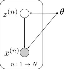
Let \(X=\\{x^{(1)}, x^{(2)}, \ldots, x^{(n)}\\}\) denote the dataset of interest, be it a set of images, a set of sound clips, or a set of document, depending on the problem at hand. The model describes a way for which the data is generated: we first sample a hidden/latent variable \(z\) from the distribution \(P(Z;\theta)\), and then sampled a data point \(x\) from the distribution \(P(X\|z;\theta)\) given the latent variable. The two probabilities are defined as we like and are given as part of the graphic models. Here we assume that the two probabilities are parameterized by a set of variables \(\theta\), although in general we could merge it as part of latent variable \(Z\) as well (as a global latent variable, the value of which is shared among all data samples), if there is a prior distribution for \(\theta\). It is worth noting that the \(P(Z;\theta)\) and \(P(X\|Z;\theta)\) could be further factorized, whichever way we design them to be, however, in this article we will just focus on the general setting.
There are two intertwined problems associated with this form of generative models: density estimation, and Bayesian inference. For the problem of density estimation, we want to estimate the probability that the model assigns to all the data \(X\) we are given in training, or more precisely \(p(X; \theta)\). The value of \(p(X; \theta)\) explains how likely it is for the model to generate the given training data. The larger the \(p(X; \theta)\), the better our model explains the existing data. For models that are parameterized by \(\theta\), fitting the model to best match the training data amounts to finding a value of \(\theta\) that maximize the density \(p(X; \theta)\).
For the problem of Bayesian inference, we want to infer the posterior probability of the unobserved hidden/latent variable given the observed data, or more precisely \(p(Z\|X;\theta)\). It is easy to see that these two problems are naturally intertwined from Bayes rule: \(p(Z\|X) = \frac{p(X\|Z)p(Z)}{P(X)}\): since \(p(X\|Z)\) and \(p(Z)\) are already given as part of the model assumption, if we solve one of the two problems, then the other one can be solved as well. Conceptually, the solution to the problems can be viewed as trying to find a reverse graph in the generative model.
Let’s now take a step back and ask the question: why do we bother with the introduction of latent/hidden variable? Can we just propose a model that captures \(p(X;\theta)\) directly, and save the trouble of Bayesian inference for the latent variable all together? Anyway, even with the direct characterization of \(p(X;\theta)\), the discussion above should still hold: the larger the \(p(X;\theta)\), the better our model explains the given data, and with a good model we can apply sampling to generate artificial data.
The benefits of the hidden/latent variables are two-fold:
- The adoption of hidden/latent variables allows one to construct complex marginal data distributions \(p(X)\) from simple and easy to evaluate distribution functions. For example, with \(p(Z;\theta)\) being the multinomial distribution and \(p(X\|Z;\theta)\) being the normal distribution, we arrive at the Gaussian mixture model \(p(X;\theta)=\int P(X\|Z;\theta)P(Z;\theta)dZ\), which can characterize a wide range of complex distribution and has significantly more expressiveness power compared with just Gaussian or multinomial distribution alone. It is evident that a model that characterizes more complex distributions can better fit the data, especially with the high-dimensional complicated data we are usually focusing on.
- The hidden/latent variables can be viewed as general features extracted from the data, which can be utilized for any downstream tasks. The hidden/latent variables normally has much lower dimension compared with the data itself, and they represent low-dimensional message that conveys condensed information regarding the corresponding data. If a model can fit the data well, meaning that the likelihood is high for the model to generate the training data by sampling \(X\) conditioned on a sampling of \(Z\), then one can argue that \(Z\) should capture the essence of the data. It is interesting to note how the above two points echo the previous discussion regarding the inter-connection between density estimation and Bayesian inference.
In the Bayesian inference problem, as stated before, the task is to find the posterior distribution of the unobserved variable \(Z\) given then observed variable \(X\). Instead of tackling this problem head on by deriving \(p(Z\|X;\theta)=\frac{p(X\|Z;\theta)p(Z;\theta)}{\int p(X\|Z;\theta)p(Z;\theta)dZ}\), which is often intractable, let us introduce another distribution \(q(Z)\) with the goal of mimicking \(p(Z\|X;\theta)\), and look at what the KL divergence between the two could decompose into:
\[\begin{align*} &\text{KL}{\big(}q||p(Z|X;\theta){\big)}\\ =&\int q(Z) \ln \frac{q(Z)}{p(Z|X;\theta)}dZ\\ =&\int q(Z) \ln \frac{q(Z)}{P(Z|X;\theta)}\frac{p(X;\theta)}{p(X;\theta)}dZ\\ =&\int q(Z) \ln \frac{q(Z)p(X;\theta)}{P(Z,X;\theta)}dZ\\ =&\int q(Z) \ln p(X;\theta)dZ-\int q(Z) \ln \frac{P(Z,X;\theta)}{q(Z)}dZ\\ =&\ln p(X;\theta)-\int q(Z) \ln \frac{P(Z,X;\theta)}{q(Z)}dZ. \end{align*}\]Making the short-hand notation of
\[\begin{align*} \mathcal{L}(q,\theta)=\int q(Z) \ln \frac{P(Z,X;\theta)}{q(Z)}dZ, \end{align*}\]we can simplify the above equation as
\[\begin{align*} \ln p(X;\theta) = \text{KL}{\big(}q||p(Z|X;\theta){\big)} + \mathcal{L}(q,\theta). \end{align*}\]The above equation is the cornerstone for a broad range of variational methods, which we will keep coming back to for later posts. Let’s stare at it for a while, observe it from different angles, and learn to appreciate its elegancy.
We should first observe that the three terms have fixed polarity: KL divergence is always nonnegative, whereas the log-likelihood term on the LHS of the equation, as well as the expression \(\mathcal{L}(q,\theta)\) is always non-positive. At first glance into the definition of \(\mathcal{L}\), it may look like it can be written in the form of negative KL divergence. However, one should note that \(P(Z,X;\theta)\) is not a proper probability on \(Z\) as \(\int p(X,Z;\theta)dZ = p(X;\theta)<1\).
Given that the KL divergence term is always nonnegative, \(\mathcal{L}(q,\theta)\) yield a lower bound on the log-likelihood of the data. In precise term, we have \(\ln p(X;\theta) \geq \mathcal{L}(q,\theta)\).
The term \(\mathcal{L}(q,\theta)\) can be viewed as a functional that maps a probability distribution function into a value. Since the analysis and optimization of functional falls into the realm of calculus of variations, the distribution function \(q\) itself is often called the variational distribution, and the lower bound \(\mathcal{L}(q,\theta)\) is referred to as the variational lower-bound.
It is important to realize that the above equation is another manifestation of the inter-connection between the data likelihood \(p(X;\theta)\) and the posterior distribution of latent variable \(p(Z\|X;\theta)\), this time linked through the variational distribution function \(q\). For a fixed parameter \(\theta\), if we increase the variational lower bound \(\mathcal{L}(q,\theta)\) by adjusting \(q\), then the updated lower-bound is closer to the log-likelihood of the data. At the same time, since an increment in \(\mathcal{L}(q,\theta)\) would infer a decrement of \(\text{KL}(q\|\|p(Z\|X;\theta))\), we know that the updated variational distribution \(q\) is closer to the true posterior distribution measured in KL divergence. To precisely capture these observations, we arrive at the following two equations
\[\begin{align*} \ln p(X;\theta) &= \max_{q}\mathcal{L}(q,\theta)\\ p(Z|X;\theta) &= \arg\max_{q}\mathcal{L}(q,\theta). \end{align*}\]This is the core of variational inference: with an introduction of a variational distribution \(q\), we can turn both the log-likelihood calculation (i.e., density estimation) problem and the Bayesian inference problem into an optimization problem, and attack it with different optimization algorithms. This inference-optimization duality provides a very powerful tool. It is the backbone of many of the variational inference related methods such as expectation-maximization, mean-field approximation, and variational auto-encoder, which we will discuss in details in the subsequent posts.
As a closing note we list two alternative proofs for the variational lower-bound below.
\[\begin{align*} &\ln p(X;\theta)\\ =&\ln\frac{p(X,Z;\theta)}{p(Z|X;\theta)}\\ =&\int q(Z)\ln\frac{p(X,Z;\theta)}{p(Z|X;\theta)}dZ\\ =&\int q(Z)\ln\frac{p(X,Z;\theta) q(Z)}{p(Z|X;\theta) q(Z)}dZ\\ =&\int q(Z)\ln\frac{p(X,Z;\theta)}{q(Z)}dZ+\int q(Z)\ln\frac{q(Z)}{p(Z|X;\theta)}dZ.\\ =&\mathcal{L}(q,\theta) + \text{KL}{\big(}q||p(Z|X;\theta){\big)}. \end{align*}\] \[\begin{align*} &\ln p(X;\theta)\\ =&\ln \int p(X,Z;\theta)dZ\\ =&\ln \int q(Z)\frac{p(X,Z;\theta)}{q(Z)}dZ \\ \geq & \int q(Z)\ln\frac{p(X,Z;\theta)}{q(Z)}dZ. \end{align*}\]