Quantization for Neural Networks
This post is a guided walkthrough of the paper A White Paper on Neural Network Quantization [Nagel et al. 2021], with additional illustrations and explanations. The same material can be found in the paper and the references therein; you are highly encouraged to read the paper directly for deeper treatment of individual topics.
Quantization of neural network models enables fast inference using efficient fixed point operations in typical AI hardware accelerators. Compared with floating point inference, it leads to less storage space, smaller memory footprint, lower power consumption, and faster inference speed, all of which are essential for practical edge deployment. It is thus a critical step in the model efficiency pipeline. In this post, based on [Nagel et al. 2021], we provide a detailed guide to network quantization.
We start off with the basics in the first section by going through the conversion of floating point and fixed point representations and introducing necessary notations. We then show how fixed point arithmetic works in a typical hardware accelerator and how to simulate it using floating point operations. Finally, we define the terminology of Post-Training-Quantization (PTQ) and Quantization-Aware-Training (QAT).
The second section covers one baseline method for range estimation, followed by three techniques to improve PTQ performance, with some also serving as a necessary step to get good initialization for QAT.
In the last part, we go over the recommended pipeline and practices of PTQ and QAT as suggested by the white paper [Nagel et al. 2021] and discuss how special layers other than Conv/FC can be handled. Here’s an outline.
- TOC
Quantization basics
Conversion of floating point and fixed point representation
Fixed point and floating point are different ways of representing numbers in computing devices. Floating point representation is designed to capture fine-grained precision (by dividing the bit field into mantissa and exponent) with high bit-width (typically 32 bits or 64 bits), whereas fixed point numbers live on a fixed width grid that are typically much coarser (typically 4, 8, 16 bits). Due to its simplicity, the circuitry for fixed point arithmetic can be much cheaper, simpler, and more efficient than its floating point counterpart. The term network quantization refers to the process of converting neural network models with floating point weights and operations into ones with fixed point weights and operations for better efficiency.
The figure below describes how the conversion from a floating point number to a fixed point integer can be done. Let us label the start and the end of the fixed point integer number as \(n\) and \(p\). For signed integer with bit-width of \(b\), we have \([n, p]=[-2^{b-1}, 2^{b-1}-1]\); for unsigned integer \([n, p]=[0, 2^{b}-1]\). In this simple example \(b=4\), which gives us 16 points on the grid.
Assume that we have a conversion scheme that maps a floating point \(0\) to an integer \(z\), and \(s\) to \(z+1\). The mapping of floating point number \(x\) to its fixed point representation \(x_\text{int}\) can be described as
\[\begin{align} x_\text{int} = \texttt{clamp}(\lfloor x/s \rceil + z; n, p),\label{eq:xint_x} \end{align}\]where \(\lfloor\cdot\rceil\) denotes rounding-to-nearest operation and \(\texttt{clamp}(\cdot: n, p)\) clips its input to within \([n, p]\). \(s\) and \(z\) are often referred to as scale and offset.
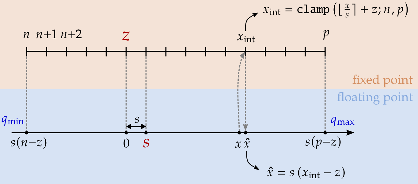
The integer \(x_\text{int}\), when mapped back to the floating point axis, corresponds to
\[\begin{align} \hat{x} = s\left(x_\text{int} - z\right).\label{eq:xhat_xint} \end{align}\]By combining the two equations, we can express the quantized floating point value \(\hat{x}\) as
\[\begin{align} \hat{x} =& s \left(\texttt{clamp}\left(\left\lfloor x/s\right\rceil +z; n, p\right)-z\right) \notag\\ =& \texttt{clamp}\left(s\left\lfloor x/s \right\rceil; s(n-z), s(p-z)\right) \notag\\ =& \texttt{clamp}{\Big(}\underbrace{s\left\lfloor x/s \right\rceil}_{\substack{\text{rounding}\\\text{error}}}; \underbrace{q_\text{min}, q_\text{max}}_{\substack{\text{clipping}\\\text{error}}}{\Big)}. \label{eq:x_hat} \end{align}\]Here we denote \(q_\text{min}\triangleq s(n-z)\) and \(q_\text{max}\triangleq s(p-z)\) as the floating point values corresponding to two limits on the fixed point grid. The quantization error \(x-\hat{x}\) comes from two competing factors: clipping and rounding. Increasing \(s\) reduces the clipping error at the cost of increased rounding error. Decreasing \(s\) reduces rounding error at the cost of a higher chance of clipping. This is referred to as range and precision tradeoff.
Before diving into the arithmetic, let us clarify what each symbol represents and what we can and cannot control. To avoid getting “lost in notation” for the many notations we introduced (\(n\), \(p\), \(b\), \(z\), \(s\), \(q_\text{min}\), \(q_\text{max}\), \(x\), \(\hat{x}\), \(x_\text{int}\)), it is important to keep the following in mind:
-
\(n\), \(p\), and \(b\) are determined by the integer type that is available to us. They describe the hardware constraints and are not something we can control (nor is there a need to control them!)
- For 8-bit signed integer we have \(n=-128\) and \(p=127\)
- For 8-bit unsigned integer we have \(n=0\) and \(p=255\)
- For bit-width of \(b\), we have \(p-n+1 = 2^b\)
-
Either \((s, z)\) or \((q_\text{min}, q_\text{max})\) uniquely describes the quantization scheme. Together they are redundant since one can derive the other. When we talk about quantization parameters, we refer to either \((s, z)\), or equivalently \((q_\text{min}, q_\text{max})\), since there are only two degrees of freedom in \((s, z, q_\text{min}, q_\text{max})\).
- Derive \((q_\text{min}, q_\text{max})\) from \((s, z)\):
- \(q_\text{min} = s(n-z)\).
- \(q_\text{max} = s(p-z)\).
- Derive \((s, z)\) from \((q_\text{min}, q_\text{max})\):
- \(s = (q_\text{max} - q_\text{min}) / 2^b\).
- \(z = n - q_\text{min}/s = p - q_\text{max}/s\).
- \(z=0\) is referred to as symmetric quantization
- Note that symmetric quantization does not imply that we have equal number of grid points on either side of integer \(0\), but rather just the fact that floating point \(0\) is mapped to integer \(0\) in the fixed point representation
- Derive \((q_\text{min}, q_\text{max})\) from \((s, z)\):
-
Among the different variables, \(z\) and \(x_\text{int}\) are fixed point numbers whereas \(x\), \(\hat{x}\), \(s\) are floating point numbers
- We want to carry out all operations in the fixed point domain, so ideally only offset \(z\) and \(x_\text{int}\) should be involved in hardware multiplication and summation.
-
The fact that floating point \(0\) maps to an integer \(z\) ensures that there is no quantization error in representing floating point \(0\)
- This guarantees that zero-padding and ReLU do not introduce quantization error
An important take-away here is that there are two equivalent definitions of quantization parameters:
- Quantization parameters are either \((s, z)\) or \((q_\text{min}, q_\text{max})\)
- In the context of QAT, we talk about \((s, z)\) more as they are directly trainable
- In the context of PTQ, \((q_\text{min}, q_\text{max})\) is used more often
- Range estimation refers to the estimation of \((q_\text{min}, q_\text{max})\)
Fixed point arithmetic
Now that we have covered how to map numbers from floating point to fixed point format, we will show how we can use fixed point arithmetic to approximate floating point operations.
Let’s first take a look at an easy case of scalar multiplication \(y = wx\), and denote the quantization parameters of \(w, x, y\) as \((s_w, z_w), (s_x, z_x), (s_y, z_y)\). From Equation \eqref{eq:xhat_xint}, the quantized version of \(w\) and \(x\) can be expressed as
\[\begin{align*} \hat{w} =& s_w(w_\text{int} - z_w)\\ \hat{x} =& s_x(x_\text{int} - z_x)\\ \end{align*}\]The product of \(wx\) can then be approximated by \(\hat{w}\hat{x}\). In what follows we will highlight fixed point numbers as blue to make it clear which of the operations are carried out in fixed point domain.
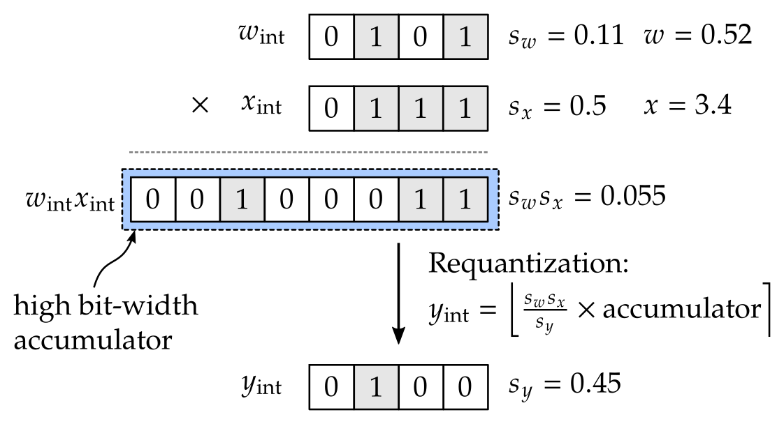
\[\begin{align*} wx \approx& \hat{w}\hat{x} \\ =& s_w({\color{blue}w_\text{int}} - {\color{blue}z_w})*s_x({\color{blue}x_\text{int}} - {\color{blue}z_x})\\ =& s_w s_x \left[ ({\color{blue}w_\text{int}}-{\color{blue}z_w})({\color{blue}x_\text{int}}-{\color{blue}z_x})\right] \\ =& \underbrace{s_w s_x}_{\substack{\text{scale of}\\\text{product}}} {\color{blue}\big[} {\color{blue}w_\text{int} x_\text{int}} - \underbrace{\color{blue}z_wx_\text{int}}_{\substack{\text{input }x\\\text{dependent}}} - \underbrace{\color{blue}w_\text{int}z_x + z_wz_x}_{\substack{\text{can be}\\\text{pre-computed}}} {\color{blue}\big]} \end{align*}\]It should be clear that all terms inside the square bracket above can be carried out in fixed point operations. Since integer multiplication will inflate bit-width (the product of two 8-bit numbers will take up 16 bits), and we also need to accumulate different terms, the result inside the bracket is typically stored in high bit-width accumulator (e.g., 32-bit accumulator).
We are not done yet – we still need to fit \(\hat{w}\hat{x}\) to the quantization grid chosen for \(y\). In other words, we need to map it to the fixed point format indicated by \((s_y, z_y)\) using Equation \eqref{eq:xint_x}, a step referred to as requantization:
\[\begin{align*} y_\text{int} =& \texttt{clamp}\left(\left\lfloor \frac{\hat{w}\hat{x}}{s_y} \right\rceil + z_y; n, p\right)\\ =& \texttt{clamp}\left(\left\lfloor \frac{s_w s_x}{s_y}\times{\color{blue}\text{Accumulator}} \right\rceil + z_y; n, p\right). \end{align*}\]In the figure below, we illustrate an example when \(z_w\), \(z_x\), and \(z_y\) are all \(0\).
The problem here is that \(\frac{s_w s_x}{s_y}\) is a floating point number, and we need to multiply it by the fixed point value in the high bit-width accumulator. This can be carried out in hardware if we approximate \(\frac{s_w s_x}{s_y}\) with the form of \({\color{blue}a}2^{n}\) where \({\color{blue}a}\) is a fixed point number and \(n\) is an integer, in which case requantization can be efficiently done by the multiplication of two fixed point numbers (value in the high bit-width accumulator, and \(a\)) followed by a bit-shift. How this operation is carried out can be hardware specific. The procedure of requantization is also described in Equation (5) and (6) in [Jacob et al. 2018].
Next we generalize the simple case of scalar multiplication to matrix-vector products with bias \(y = W x + b\). For the weight matrix \(W\), the \(i^\text{th}\) row is responsible for computing the \(i^\text{th}\) output element, which is referred to as output channel, expressed as follows:
\[\begin{align} y_i =& \sum_{j}W_{ij}x_j + b_i\notag\\ \approx& \sum_{j}\hat{W}_{ij}\hat{x}_j + \hat{b}_i \notag\\ =& \sum_{j} s_i^w \left(W_{ij}^\text{int} - z_i^w\right) s^x \left(x_j^\text{int}- z^x\right) + s_i^ws^x b_i^\text{int}\notag\\ =& s_i^ws^x {\bigg[} \sum_{j}{\big(} W_{ij}^\text{int}x_j^\text{int} - z_i^wx_j^\text{int} - W_{ij}^\text{int}z^x + z_i^wz^x {\big)} + b_i^\text{int} {\bigg]}\notag\\ =& s_i^ws^x {\color{blue}\bigg[} \underbrace{\color{blue}\sum_{j}{\big(} W_{ij}^\text{int}x_j^\text{int}{\big)}}_{\substack{\text{Multiply-Accumulate}\\\text{(MAC)}}} - \underbrace{\color{blue}\sum_{j}{\big(}z_i^wx_j^\text{int}{\big)}}_{\substack{\text{No-op if}\\\text{ weight offset is }0}} + \underbrace{\color{blue}\sum_{j}{\big(}- W_{ij}^\text{int}z^x + z_i^wz^x {\big)} + b_i^\text{int}}_{ \substack{\text{Can be pre-computed and }\\\text{pre-loaded to the accumulator}}} {\color{blue}\bigg]} \label{eq:y_i} \end{align}\]A few remarks are in order:
- Treatment of bias quantization:
- It should be clear that in order for the bias to be easily added to the accumulator, we should fix its scale to be \(s_i^b = s_i^ws^x\). In other words, the scale of bias is not a free variable that we can control.
- Since \(b_\text{int}\) can be directly added to the high bit-width accumulator, we normally don’t need to be concerned regarding clipping error of bias quantization.
- For the four terms inside the square bracket
- The last two are not data dependent and can be pre-computed, merged with bias, and pre-loaded to the accumulator together, with no additional inference cost.
- The second one, however, is data dependent, but vanishes if weight offset \(z_i^w\) is zero. To save compute, a common approach is to keep weight quantization to be symmetric (i.e., \(z_i^w=0\)) so that this term goes away.
- The output \(y\) typically goes through nonlinear activation functions
- Some activation functions such as ReLU can be directly applied in the accumulator before requantization is applied.
A common design choice is to have symmetric weight quantization (\(z^w=0\)) and asymmetric activation quantization to avoid the data dependent term.
Per-tensor vs per-channel quantization
Equation \eqref{eq:y*i} describes the operations needed to obtain the result of the \(i^\text{th}\) output channel. One assumption made is that weights for the same output channel (\(W*{i\cdot}=W*{i,1}, W*{i,2}, \ldots\) corresponds to the \(i^\text{th}\) output channel) share the same quantization parameters, denoted as \(s_i^w\) and \(z_i^w\), and that all the elements in the input tensor \(x=[x_1, x_2, \ldots]\) share the same quantization parameters denoted as \(s^x\) and \(z^x\). In this part we review different choices of quantization granularity.
One common setting is to have a single set of quantization parameters for the entire weight tensor, which corresponds to figure (a) illustrated below. This is referred to as per tensor quantization. In this case, all the output channels of the weights share the same scaling factor \(s^ws^x\), and thus the requantization operation is uniform across all the output channels.
One problem with this setting is that in practice, weights from different output channels could have a wide difference in their dynamic ranges. E.g., weights in the first channel may range from \(-500.0\) to \(500.0\) while the second from \(-1.0\) to \(1.0\). If we pick quantization parameters to \([-500, 500]\) in 8-bit, the second channel will be completely quantized away (i.e., quantized to \(0\), aka underflow), losing all its information. On the other hand, if we fit the range to \([-1, 1]\), the first channel will suffer from huge clipping error. In one of the later sections a technique called cross layer equalization is introduced to alleviate this issue by trying to equalize range for different channels.
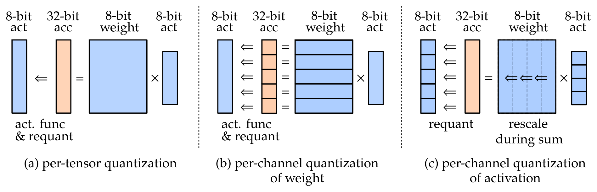
A more flexible setting is to allow different channels to be quantized differently [Krishnamoorthi 2018], referred to as per-channel quantization of weight. This is the setting captured by figure (b) above, and is the case described in Equation \eqref{eq:y_i} where \(s_i^w\) can be different for different output channels with index \(i\). The hardware implication for this setting is that requantization is no longer uniform across different output channels. This scheme would save us from the varying dynamic range issue mentioned before, but not every hardware platform supports this setting.
Both (a) and (b) assume that the activation is quantized in a per-tensor fashion. The alternative option of per-channel quantization of activation, as illustrated in Figure (c), is extremely hard to handle in hardware. In this setting, the accumulator needs to be rescaled for each input dimension. As is evident from Equation \eqref{eq:y*i}, having a per-channel quantization of activation implies that the scaling factor for activation should be denoted as \(s*{\color{red}j}^x\), and as a result we can no longer factor \(s_i^{w}s^x_j\) outside of the summation across input dimension \(j\), meaning that each multiply-and-accumulation would require a rescaling operation. Due to its hardware difficulty, most fixed-point accelerators do not support this setting.
- (a) per-tensor quantization
- base setting supported by all fixed point accelerators
- can suffer from large quantization error due to varying dynamic ranges across different output channels of the weight
- (b) per-channel quantization of weights
- also simply referred to as per-channel quantization
- increasingly standard, though not universally supported across hardware
- (c) per-channel quantization of activation
- as of now this is not generally considered as a viable solution due to the difficulty in hardware implementation
Quantization simulation and gradient computation
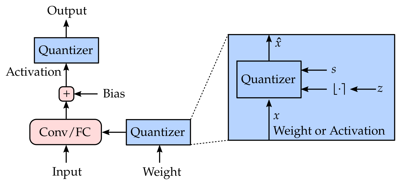
Fixed point operation can be simulated with floating-point training if we map the weight \(W\) and activation \(x\) values to their quantized versions \(\widehat{W}\) and \(\hat{x}\). The mapping is described in Equation \eqref{eq:x_hat} and re-stated below.
\[\begin{align} \hat{x} =& \texttt{clamp}{\bigg(}\underbrace{s\left\lfloor x/s \right\rceil}_{\substack{\text{rounding}\\\text{error}}}; \underbrace{\overbrace{s(n-z)}^{q_\text{min}}, \overbrace{s(p-z)}^{q_\text{max}}}_{\text{clipping error}}{\bigg)} = \left\{ \begin{array}{ll} s\left\lfloor x/s \right\rceil & \text{if } q_\text{min} \leq x \leq q_\text{max} \\ s(n-z) & \text{if } x < q_\text{min} \\ s(p-z) & \text{if } x > q_\text{max} \end{array} \right.\label{eq:x_hat_re} \end{align}\]The schematic below illustrates how simulated quantization described by this equation above can be added to a typical network layer.
These gradients are needed when training with simulated quantization (QAT), which we return to later. From Equation \eqref{eq:x_hat_re} we can derive the gradient of the quantized value with respect to the input as well as the quantization parameters (\(s\) and \(z\)) as follows. In order to back-propagate through rounding \(\lfloor\cdot\rceil\), the straight-through estimator \(\partial \lfloor x \rceil/\partial x \approx 1\) is used (denoted as \(\overset{\text{st}}{\approx}\) below).
\[\begin{align} \frac{\partial \hat{x}}{\partial x} =& \left\{ \begin{array}{ll} s \frac{\partial}{\partial x}\left\lfloor x/s\right\rceil \overset{\text{st}}{\approx} 1 &\text{if } q_\text{min} \leq x \leq q_\text{max} \\ 0 & \text{if } x < q_\text{min} \\ 0 & \text{if } x > q_\text{max} \end{array} \right.\label{eq:d_hatx_dx}\\ \frac{\partial \hat{x}}{\partial s} =& \left\{ \begin{array}{ll} \left\lfloor x/s \right\rceil + s \frac{\partial}{\partial s} \left\lfloor x/s \right\rceil \overset{\text{st}}{\approx} \left\lfloor x/s \right\rceil - x/s &\text{if } q_\text{min} \leq x \leq q_\text{max} \\ n - z & \text{if } x < q_\text{min} \\ p - z & \text{if } x > q_\text{max} \end{array} \right. \label{eq:d_hatx_ds}\\ \frac{\partial \hat{x}}{\partial z} =& \left\{ \begin{array}{ll} 0 &\text{if } q_\text{min} \leq x \leq q_\text{max} \\ -s & \text{if } x < q_\text{min} \\ -s & \text{if } x > q_\text{max} \end{array} \right. \label{eq:d_hatx_dz} \end{align}\]Post-Training-Quantization (PTQ) vs Quantization-Aware-Training (QAT)
There are two different model quantization methodologies: Post Training Quantization (PTQ) and Quantization Aware Training (QAT).
In post training quantization (PTQ), a well-trained floating-point model is converted to a fixed point one without any end-to-end training. The task here is to find ranges (quantization parameters) for each weight and activation, and this is done either without any data or with only a small representative unlabelled dataset, which is often available. Since no end-to-end training is involved, it decouples model training from model quantization, which allows quantization to be applied entirely post-training, with no need for retraining or fine-tuning.
Quantization-aware training (QAT), by contrast, integrates quantization operations as part of the model, and trains the quantization parameters together with the model’s neural network parameters, where the backward flow through the quantization operation is described in the previous section. Here we need access to the full training dataset. Setting up the training pipeline that involves simulated quantization can be a difficult process and requires more effort than PTQ, but it often results in close-to-floating-point performance, sometimes even with very low bit-width.
In the next section, we first go over some baseline quantization range estimation methods, and then describe three techniques that boost PTQ performance. Keep in mind that some of the PTQ techniques can lead to better initialization for QAT and thus can be very relevant in the QAT context as well.
Quantization techniques
Range Estimation Methods
This part covers how the range (\(q_\text{min}, q_\text{max}\)) of weight and/or activation can be estimated. As noted before, \((q_\text{min}, q_\text{max})\), or equivalently \((s, z)\), uniquely determine the quantization scheme for a given fixed-point format \((b, n, p)\). All these approaches need some statistical information of the data to be quantized. For weight, this is readily available, and for activation, it can be estimated with a small set of representative input data.
Min-Max
To avoid any clipping error, we can set \(q_\text{min}\) and \(q_\text{max}\) to the min and max of the tensor to be quantized.
\[\begin{align*} q_\text{min} =\min x\\ q_\text{max} =\max x \end{align*}\]The downside of this approach is that a large rounding error may be incurred if there are strong outliers in the min/max values.
MSE
To strike the right balance between range and precision, we can instead minimize the mean-square-error (MSE) between the quantized values and the floating point ones,
\[\underset{q_\text{min},q_\text{max}}{\arg\min} \|x-\hat{x}\|_F^2.\][Banner et al. 2019] introduced an analytical approximation of the above objective when \(x\) follows either Laplace or Gaussian distribution (or one-sided Gaussian/Laplace if \(x\) is the output of a ReLU activation). Alternatively, a simple grid search also works.
Cross-Entropy
For models with the last layer being a softmax, we can derive quantization parameters of the last layer activation (which are logits) by minimizing the error in probability space, instead of MSE.
\[\underset{q_\text{min},q_\text{max}}{\arg\min}\text{ }\texttt{CrossEntropy}(\texttt{softmax}(x),\texttt{softmax}(\hat{x}))\]BatchNorm
In layers with BatchNorm, we can use its learned parameters (mean-shift \(\beta\) and learned scale \(\gamma\), following the convention in the source paper) to approximate min and max as \(q_\text{min}\approx \beta - \alpha\gamma\) and \(q_\text{max} \approx \beta + \alpha\gamma\) where \(\alpha=6\) is recommended.
One minor detail for all the above approaches is that the value of \(q_\text{min}\) and \(q_\text{max}\) needs to be tweaked to ensure that the corresponding offset \(z\) is an integer value on the grid.
Empirically, MSE-based method is the most robust across different models and bit-width settings, and thus is the recommended method for range estimation. For logit activation, Cross-Entropy based method can be beneficial especially in low bit-width regime (4-bit or below).
Cross Layer Equalization
We have mentioned that per-tensor quantization of weight can be problematic when weights for different output channels have significantly different ranges. The issue can be side-stepped using per-channel quantization of weights, but not all hardware supports it.
It turns out there is an elegant way to re-scale weights across layers without changing the model’s output, making it much more amenable to per-tensor quantization. The technique is called Cross Layer Equalization (CLE), proposed by [Nagel et al. 2019] and [Meller et al. 2019]. Let’s go over it.
A linear map \(f\) satisfies two properties: (1) additivity: \(f(a+b)=f(a)+f(b)\), and (2) scale equivariance: \(sf(a) = f(sa)\) (scaled input leads scaled output). Some of the most commonly used nonlinear activation functions such as ReLU or leaky ReLU only give up the first property but still have the second property hold for any positive scaling factor \(s\).
The scale equivariance property allows us to redistribute the scaling of weights of two adjacent layers even with the activation function in the middle. In the naive scalar example, this can be seen as
\[w^{(2)}f\left(w^{(1)}x\right) = sw^{(2)}f\left(\frac{w^{(1)}}{s} x\right).\]For the general case of two consecutive Conv or FC layers (weights denoted as \(W^{(1)}, W^{(2)}\)) with a scale-equivariant nonlinearity in the middle (denoted as \(f\)), we can apply a scaling of \(s_i\) on the \(i^\text{th}\) input channel of \(W^{(2)}\) (\(W^{(2)}_{\cdot i}\)) and a scaling of \(1/s_i\) on the \(i^\text{th}\) output channel of \(W^{(1)}\) (\(W^{(1)}_{i \cdot}\)) without changing the output.
\[\begin{align*} &W_{c_3\times c_2}^{(2)} f\left( W_{c_2\times c_1}^{(1)}x\right)\\ =&\left[W_{\cdot 1}^{(2)},\ldots,W_{\cdot c_2}^{(2)}\right] f\left(\left[ \begin{array}{c} W_{1\cdot}^{(1)} \\ \vdots \\ W_{c_2\cdot}^{(1)} \\ \end{array} \right]x\right)\\ =&\left[W_{\cdot 1}^{(2)},\ldots,W_{\cdot c_2}^{(2)}\right] \left[ \begin{array}{c} f(W_{1\cdot}^{(1)}x) \\ \vdots \\ f(W_{c_2\cdot}^{(1)}x) \\ \end{array} \right]\\ =&\sum_{i:1\to c_2} W_{\cdot i}^{(2)}f\left(W_{i\cdot}^{(1)}x\right)\\ =&\sum_{i:1\to c_2} W_{\cdot i}^{(2)} s_i f\left(\frac{W_{i\cdot}^{(1)}}{s_i}x\right) \end{align*}\]This is illustrated in the figure below, where we take as an example two 1x1 convolutions with a ReLU in between.
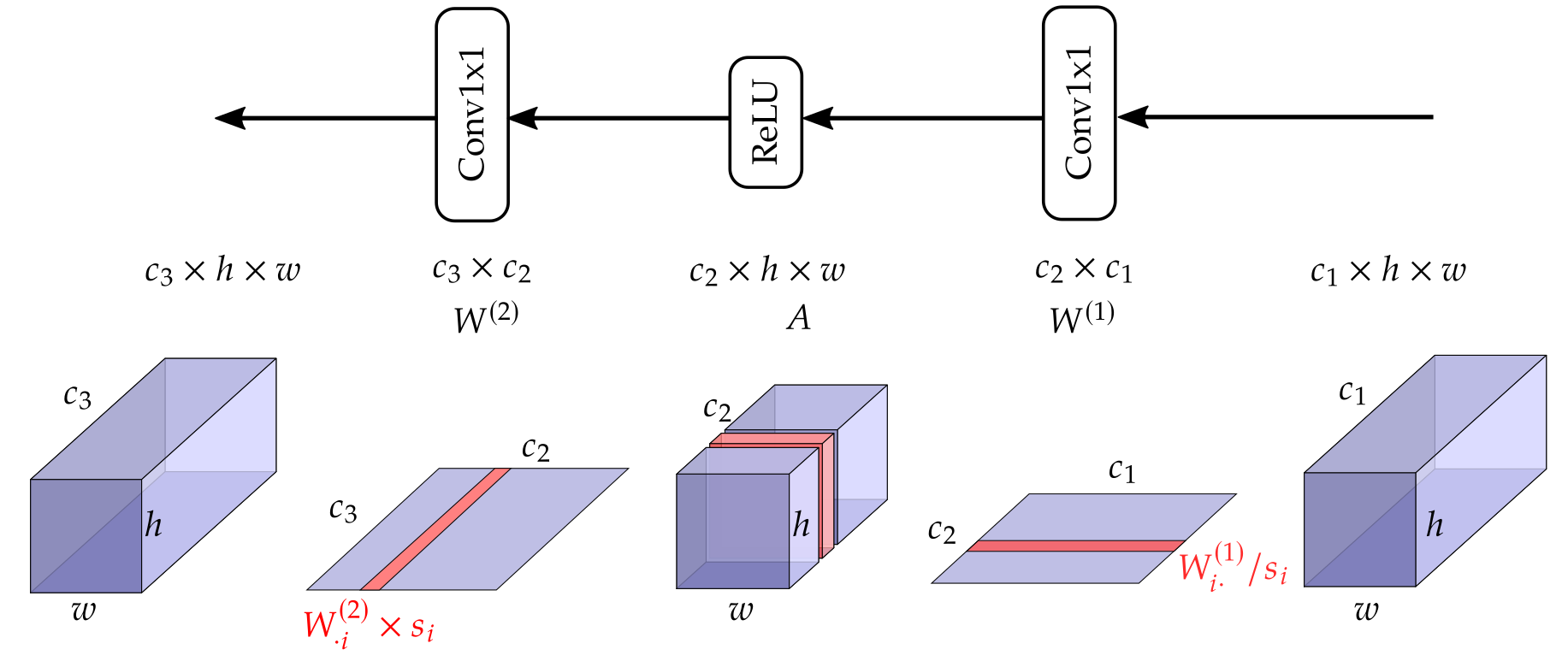
Intuitively, we want to redistribute the magnitude of weights between the two weight tensors in such a way that the maximum magnitude can be equalized. In other words, whenever the range of \(W^{(1)}_{i\cdot}\) is larger than that of \(W^{(2)}_{\cdot i}\), there is an incentive to down scale \(W^{(1)}_{i\cdot}\) and up scale \(W^{(2)}_{\cdot i}\) to the point that they match in their range. With this intuition in mind, we can find the scaling factors to be applied for each channel \(i\) as (output channel of \(W^{(1)}\) and input channel of \(W^{(2)}\)):
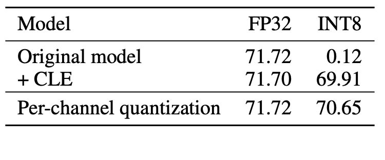
\[\begin{align*} &\max\left| W_{\cdot i}^{(2)} s_i \right| = \max\left|\frac{W_{i\cdot}^{(1)}}{s_i}\right| \\ \Longrightarrow & \max\left| W_{\cdot i}^{(2)}\right| s_i = \max\left|W_{i\cdot}^{(1)}\right|/s_i \\ \Longrightarrow & s_i = \sqrt{\frac{ \max\left|W_{i\cdot}^{(1)}\right| }{ \max\left| W_{\cdot i}^{(2)}\right| }}. \end{align*}\]Cross layer equalization with the scaling factor derived as above is a highly effective way to boost performance of PTQ when per-tensor quantization of weight is applied. It is especially critical for models that use depth-wise separate convolution, which empirically leads to large variation in magnitude of weights from different channels. Below is Table 3 from [Nagel et al. 2021], which shows that applying CLE on the floating point model before PTQ can fix the PTQ performance from a complete breakdown to less than 2 percent loss compared with floating point.
To summarize, CLE is a technique that adjusts weights of a floating point model so that it becomes more friendly with per-tensor quantization of weights. Some remarks below
- In the context of PTQ, CLE is a must have whenever per-tensor quantization is applied.
- In the context of QAT, CLE still is a necessary model-preprocessing step to get a good initialization of the per-tensor quantization parameters.
- A limitation for CLE is that it cannot handle pairs of layers where there is skip connection to or from the activation in the middle.
- [Meller et al. 2019] proposes to apply equalization that also takes into account the activation tensor in the middle
- To apply CLE to a deep model, the process is iterated for every pair of layers (that does not have skip connection to or from the middle layer) sequentially until convergence.
Bias Correction
Quantization of weights can lead to a shift in the mean value of the output distribution. Specifically, for a linear layer with weight \(W\) and input \(x\), the gap between the mean output of quantized weight \(\hat{W}\) and its floating point counterpart \(W\) can be expressed as \(\mathbb{E}[\hat{W}x] - \mathbb{E}[Wx] = (W-\hat{W})\mathbb{E}[x]\). Given that \(x\) is the activation of the previous layer, \(\mathbb{E}[x]\) is often non-zero (e.g., if \(x\) is the output of the ReLU activation), and thus the gap can be non-zero.
This shift in the mean can be easily corrected by absorbing \((W-\hat{W})\mathbb{E}[x]\) into the bias term (subtract \((W-\hat{W})\mathbb{E}[x]\) from bias) [Nagel et al. 2019]. Since \(W\) and \(\hat{W}\) are known after the quantization, we only need to estimate \(\mathbb{E}[x]\), which can come from two sources
- If there is a small amount of input data, it can be used to get an empirical estimate of \(\mathbb{E}[x]\)
- If \(x\) is the output of a BatchNorm + ReLU layer, we can use the batch norm statistics to derive \(\mathbb{E}[x]\)
Adaptive Rounding
In PTQ, after the quantization range \([q_\text{min}, q_\text{max}]\) (or equivalently, step size \(s\) and offset \(z\)) of a weight tensor \(W\) is determined, the weight will be rounded to its nearest value on the fixed-point grid. Rounding to the nearest quantized value is such an apparently right operation that we don’t think twice about it. However, there is a valid reason why we may consider otherwise.
Let us first define a more flexible form of quantization \(\widetilde{W}\) where we can control whether to round up or down with a binary auxillary variable \(V\):
\[\begin{align*} \text{Round to nearest } \widehat{W} =& s \left\lfloor W/s\right\rceil, \\ \text{Round up or down } \widetilde{W}(V) =& s \left(\left\lfloor W/s\right\rfloor + V\right). \end{align*}\]Note that we changed \(\lfloor\cdot\rceil\) into \(\lfloor\cdot\rfloor\) and ignored clamping for notational clarity. Rounding-to-nearest minimizes the mean-square-error (MSE) between the quantized values and their floating point values, i.e.,
\[\widehat{W} = \min_{V\in [0, 1]^{|V|}} \left\| W - \widetilde{W}(V) \right\|_F^2.\]Instead of minimizing MSE of the quantized weight, a better target is to minimize the MSE of the activation, which reduces the effect of quantization from an input-output standpoint:
\[\min_{V\in [0, 1]^{|V|}} \left\|f(Wx) - f\left(\widetilde{W}(V)\bar{x}\right)\right\|_F^2.\]The method of determining whether to round up or round down by optimizing the above objective is called Adaptive Rounding or AdaRound proposed by [Nagel et al. 2020]. \(\bar{x}\) is the activation with all previous layers quantized. Note that optimization of the above objective only requires a small amount of representative input data. Please refer to [Nagel et al. 2020] for details regarding how this integer optimization problem can be solved with relaxation and annealed regularization term that encourages \(V\) to converge to 0/1.
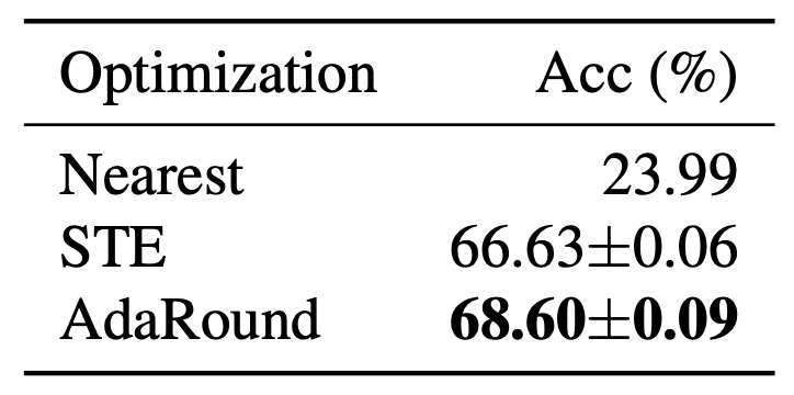
Alternatively, one can use the straight-through estimator (STE) to directly optimize for the quantized weight, which allows more flexible quantization beyond just rounding up or down. In the table below, we can see that AdaRound outperforms this STE approach, likely due to biased gradient of STE.
To summarize, AdaRound is an effective PTQ weight quantization technique, with the following characteristics/limitations:
- It requires access to a small amount of representative input data (no label needed)
- It is only a weight quantization technique
- It is applied after the range (\(q_\text{min}\) and \(q_\text{max}\), or equivalently \(s\) and \(z\)) is determined.
- When QAT is applied, AdaRound becomes irrelevant.
- AdaRound absorbs bias correction in its optimization objective (In the equations above, \(f(Wx)\) should be \(f(Wx+b)\), but we ignored \(b\) for notational clarity), so whenever AdaRound is applied, bias correction is no longer needed.
PTQ and QAT best practices
PTQ pipeline and debugging strategy
A practical PTQ workflow consists of three phases: an initial setup, a systematic debugging pass, and a final optimized pipeline.
Initial pipeline
- Add quantizer
- Symmetric weight and asymmetric activation quantization are recommended
- Symmetric is preferred for weight to avoid the second term in Equation \eqref{eq:y_i}.
- Per-tensor quantization of weight and activation
- Symmetric weight and asymmetric activation quantization are recommended
- Range estimate for weight
- MSE based range estimate is recommended
- Range estimate for activation
- MSE based range estimate is recommended
Debug steps
When the initial pipeline underperforms, the following strategy can help isolate the source of accuracy loss.
- Check if the 32-bit fixed-point model matches the performance of the floating-point model
- A bit-width of 32 gives very high precision and should match the floating-point model
- If it does not match, check the correctness of the range learning module and quantizer.
- Identify which one is the major cause of performance degradation: weight quantization or activation quantization
- (A) Use bit-width of 32 for weight quantization and the targeted bit-width for activation quantization
- (B) Use bit-width of 32 for activation quantization and the targeted bit-width for weight quantization
- Once we identify which one is more problematic, we can further identify which layer(s) are the bottleneck
- We can conduct leave-one-out analysis by quantizing all but one layer
- and/or add-one-only analysis by quantizing only a single layer
- If weight quantization causes accuracy drop
- Apply CLE as a preprocessing step before quantization
- Apply per-channel quantization if it is supported by the target hardware
- Apply AdaRound if there is a small representative unlabeled dataset available
- Apply bias-correction if the dataset is not available, but there is BN, which captures some data statistics
- If activation quantization causes accuracy drop
- Apply CLE that also takes activation range into account [Meller et al. 2019] before quantization
- Apply different range estimate methods (MSE is recommended, but for logit activation, cross-entropy based method can be applied)
- Visualize the range/distribution for problematic tensors
- Break down the range/distribution per-channel, per-dimension, and/or per-token (in sequence models)
- Set quantization to a larger bit-width for problematic layers if permitted by hardware. E.g., changing certain layers from 8-bit to 16-bit. Having heterogeneous bit-width across different layers is also often referred to as mixed-precision.
- Apply QAT
Final Pipeline
Once the root cause is identified, the following refined pipeline incorporates the relevant techniques.
- Apply CLE
- Weight only CLE
- or CLE that takes activation into account as well
- Add quantizer
- Symmetric weight quantization and asymmetric activation quantization
- Range estimate for weight
- MSE based range estimation is recommended
- Min/max can also be a good choice if per-channel quantization of weight is used
- AdaRound or bias-correction
- Adjust quantized weight/bias given a fixed range
- Range estimate for activation
- MSE based range estimation is recommended
- Cross-entropy can also be a good choice if a certain layer contains values interpreted as logits
QAT pipeline
While PTQ is performed entirely after training, QAT integrates simulated quantization into the training loop itself, allowing the model to adapt to quantization error during optimization. The PTQ techniques above — particularly CLE and MSE-based range estimation — serve as important initialization steps that make QAT more stable and efficient. The recommended QAT pipeline is as follows.
- Preprocessing of model
- Cross-layer-equalization
- Absorb BatchNorm into weights and biases of the preceding layer
- Add quantizer
- Symmetric weight quantization and asymmetric activation quantization are recommended
- Symmetric is preferred for weight because it eliminates the second term in Equation \eqref{eq:y_i}
- Per-tensor quantization of weight and activation
- Per-channel quantization of weight is preferable if supported by hardware
- Symmetric weight quantization and asymmetric activation quantization are recommended
- Range estimate
- MSE based range estimation is recommended
- They serve as initial quantization parameters
- Learn quantization parameters together with neural network parameters
- Gradient of quantization parameters can be derived from Equation \eqref{eq:x_hat_re} and are provided in Equation \eqref{eq:d_hatx_dx}, \eqref{eq:d_hatx_ds} and \eqref{eq:d_hatx_dz}.
Treatment of special layers
For addition operation and concatenation operation, we need to make sure that two activations to be added or concatenated live on the same quantization grid, i.e., we need the quantization parameters of the two activations to be the same.
So far we have covered Conv and MLP type of linear layers with simple activation functions. BatchNorm can be easily folded into the linear layer so we also understand how it can be handled. These give great coverage for typical vision models, but for the quantization of sequence/NLP models that use transformers, we also need to deal with additional non-linear operators such as LayerNorm, softmax, and GeLU. [Kim et al. 2021] addresses this challenge by proposing polynomial approximations to these operations that can be carried out easily in fixed point arithmetic. Also see [Bondarenko et al. 2021], which proposes per-embedding-group quantization for PTQ that tackles structured outliers in certain embedding dimensions of sequences. Together, these considerations provide a comprehensive foundation for deploying quantized neural networks in practice.
References
- [Nagel et al. 2021] Markus Nagel, Marios Fournarakis, Rana Ali Amjad, Yelysei Bondarenko, Mart van Baalen, Tijmen Blankevoort “A White Paper on Neural Network Quantization”, Arxiv June 2021
- [Kim et al. 2021] Sehoon Kim, Amir Gholami, Zhewei Yao, Michael W. Mahoney, Kurt Keutzer “I-BERT: Integer-only BERT Quantization”, ICML 2021
- [Bondarenko et al. 2021] Yelysei Bondarenko, Markus Nagel, Tijmen Blankevoort “Understanding and Overcoming the Challenges of Efficient Transformer Quantization”, EMNLP 2021 code
- [Nagel et al. 2020] Markus Nagel, Rana Ali Amjad, Mart Van Baalen, Christos Louizos, Tijmen Blankevoort “Up or Down? Adaptive Rounding for Post-Training Quantization”, ICML 2020
- [Nagel et al. 2019] Markus Nagel, Mart van Baalen, Tijmen Blankevoort, Max Welling, “Data-Free Quantization Through Weight Equalization and Bias Correction”, ICCV 2019
- [Meller et al. 2019] Eldad Meller, Alexander Finkelstein, Uri Almog, Mark Grobman, “Same, Same But Different: Recovering Neural Network Quantization Error Through Weight Factorization”, ICML 2019
- [Banner et al. 2019] Ron Banner, Yury Nahshan, Daniel Soudry “Post training 4-bit quantization of convolutional networks for rapid-deployment”, NeurIPS 2019
- [Jacob et al. 2018] Benoit Jacob, Skirmantas Kligys, Bo Chen, Menglong Zhu, Matthew Tang, Andrew Howard, Hartwig Adam, Dmitry Kalenichenko, “Quantization and Training of Neural Networks for Efficient Integer-Arithmetic-Only Inference“, CVPR 2018
- [Krishnamoorthi 2018] Raghuraman Krishnamoorthi, “Quantizing deep convolutional networks for efficient inference: A whitepaper ”, Arxiv 2018