Optical Flow -- An Overview
- TOC
Definition of Optical Flow
Distribution of apparent velocities of movement of brightness pattern in an image.
- Where do we need it?
- Action recognition
- Motion segmentation
- Video compression
Useful Resources
- CMU Computer Vision 16-385
- CMU Computer Vision 16-720
- Papers
- FlowNet: Learning Optical Flow with Convolutional Networks (ICCV 2015)
- FlowNet 2.0: Evolution of Optical Flow Estimation with Deep Networks (CVPR 2017)
- Optical Flow Estimation using a Spatial Pyramid Network (CVPR 2017)
- Optical Flow Estimation in the Deep Learning Age (2020/04/06)
- PWC-Net: CNNs for Optical Flow Using Pyramid, Warping, and Cost Volume (CVPR 2018)
- Iterative Residual Refinement for Joint Optical Flow and Occlusion Estimation (CVPR 2019)
- A fusion approach for multi-frame optical flow estimation (WACV 2019)
- ScopeFlow: Dynamic Scene Scoping for Optical Flow (CVPR 2020)
- MaskFlownet: Asymmetric Feature Matching with Learnable Occlusion Mask (CVPR 2020)
- RAFT: REcurrent All-Pairs Field Transforms for Optical Flow (Arxiv 2020)
Traditional Approach
Brightness Constancy Assumption
\[\begin{align*} I(x(t), y(t), t) = C \end{align*}\]Small Motion Assumption
\[\begin{align*} &I(x(t+\delta t), y(t+\delta t), t+ \delta t) = I(x(t), y(t), t) + \frac{dI}{dt}\delta t, \text{(higher order term ignored)}\\ &\text{where }\frac{dI}{dt} = \frac{\partial I}{\partial x}\frac{d x}{d t} + \frac{\partial I}{\partial y}\frac{d y}{d t} + \frac{\partial I}{\partial t}\triangleq I_x u + I_y v + I_t \triangleq \nabla^T I [u, v]^T + I_t \end{align*}\]\(\nabla I = [I_x, I_y]^T\) : spatial derivative
\(I_t\) : temporal derivative
\([u, v]\) : optical flow velocities
Brightness Constancy Equation
Combining the above two assumptions, we obtain
\[\begin{align*} \nabla I [u, v]^T + I_t = 0. \end{align*}\]How to solve Brightness Constancy Equation?
Temporal derivative \(I_t\) can be estimated by frame difference; spatial derivative \(\nabla I\) can be estimated using spatial filters. Since there are two unknowns (\(u\) and \(v\)), the system is under-determined.
Two ways to enforce additional constraints:
- Lucas-Kanade Optical Flow (1981) : assuming local patch has constant flow
- LS can be applied to solve this overdetermined set of equations
- If there is lack of spatial gradient in a local path, then the set of equations could still be under-determined. This is referred to as the
apertureproblem - If applied to only tractable patches, these are called sparse flow
- Horn-Schunck Optical Flow (1981) : assuming a smooth flow field
Formulation of Horn-Shunck Optical flow
Brightness constancy constraint/loss :
\[\begin{align*} E_d(i, j) = \left[I_x(i,j) u(i,j)+I_y(i,j)v(i,j) + I_t(i,j)\right]^2 \end{align*}\]Smoothness constraint/loss :
\[\begin{align*} E_s(i, j) = \frac{1}{4}\left[(u(i,j)-u(i+1,j))^2, (u(i,j)-u(i,j+1))^2, (v(i,j)-v(i+1,j)^2, (v(i,j)-v(i,j+1))^2\right] \end{align*}\]Solving for optical flow :
\[\begin{align*} \text{min}_{\bf{u}, \bf{v}} \sum_{i,j} E_d(i,j) + \lambda E_s(i,j) \end{align*}\]Gradient descent can be used to solve the above optimization problem.
Discrete Optical Flow Estimation
Brightness Constancy Equation assumes small motion, which is in general not the case. If the movement is beyond 1 pixel, then higher order terms in the Taylor expansion of \(I(x(t), y(t), t)\) could dominate. There are two solutions
- To reduce the resolution using coarse-to-fine architecture
- Resort to discrete optical flow estimation
For case-2, we obtain optical flow estimate by minimizing the following objective
\[\begin{align*} &E({\bf{z}}) = \sum_{i\in\mathcal{I}}D(z_i) + \sum_{(i,j)\in \mathcal{N}}S(z_i, z_j)\\ &\text{where } z_i\triangleq (u_i, v_j), \mathcal{I}\triangleq\text{set of all pixels }, \mathcal{N}\triangleq\text{set of all neighboring pixels} \end{align*}\]The above can be viewed as energy minimization in a Markov random field.
Dataset
Table 1 from FlowNet
| Entry | Frame Pairs | Frames with ground truth | Ground-truth density per frame |
|---|---|---|---|
| Middlebury | 72 | 72 | 100% |
| KITTI2012 | 194 | 194 | 50% |
| MPI Sintel | 1041 | 1041 | 100% |
| Flying Chairs | 22872 | 22972 | 100% |
| Flying Things 3D | 22872 | - | 100% |
Middlebury (link, paper)
Contains only 8 image pairs for training, with ground truth flows generated using four different techniques. Displacements are very small, typically below 10 pixels. (Section 4.1 in FlowNet)
MPI Sintel (link, paper)
Computer-animated action movie. There are three render passes with varying degree of realism
- Albedo render pass
- Clean pass (adds natural shading, cast shadows, specular reflections, and more complex lighting effects)
- Final pass (adds motion blur, focus blur, and atmospherical effect)
Contains 1064 training / 564 withheld test flow fields
KITTI (link, paper)
Contains 194 training image pairs and includes large displacements, but contains only a very special motion type. The ground truth is obtained from real world scenes by simultaneously recording the scenes with a camera and a 3D laser scanner. This assumes that the scene is rigid and that the motion stems from a moving observer. Moreover, motion of distant objects, such as the sky, cannot be captured, resulting in sparse optical flow ground truth.
Flying Chairs (link, paper)
Contains about 22k image pairs of chairs superimposed on random background images from Flickr. Random affine transformations are applied to chairs and background to obtain the second image and ground truth flow fields. The dataset contains only planar motions. (Section 3 in FlowNet 2.0)
Flying Things 3D (link, paper)
A natural extension of the FlyingChairs dataset, having 22,872 larger 3D scenes with more complex motion patterns.
Evaluation Metric
Angular Error (AE)
AE between \((u_0, v_0)\) and \((u_1, v_1)\) is the angle in 3D space between \((u_0, v_0, 1.0)\) and \((u_1, v_1, 1.0)\). Error in large flow is penalized less than errors in small flow. (Section 4.1 in link)
End Point Error (EPE)
EPE between \((u_0, v_0)\) and \((u_1, v_1)\) is \(\sqrt{(u_0-u_1)^2 + (v_0-v_1)^2}\) (Euclidean distance).
For Sintel MPI, papers also often reports detailed breakdown of EPE for pixels with different distance to motion boundaries (\(d_{0-10}\), \(d_{10-60}\), \(d_{60-140}\)) and different velocities (\(s_{0-10}\), \(s_{10-40}\), \(s_{40+}\)).
End-to-end regression based optical flow estimation
Some useful concepts
- Backward warping
\(I_1(\cdot, \cdot)\triangleq I(\cdot, \cdot, t=1), I_2(\cdot, \cdot)\triangleq I(\cdot, \cdot, t=2)\). Optical flow field \(u, v\) satisfies \(I_1(x, y) = I_2(x+u, y+v)\). In other words, \(u,v\) tells us where each pixel in \(I_1\) is coming from, compared with \(I_2\), and given \(u, v\), we know how to move around (warp) the pixels in \(I_2\) to obtain \(I_1\). Here \(I_1\) is often referred to as the source image and \(I_2\) the target image – flow vector is defined per source image. Specifically, we can define a warp operation as below
- Compositivity of backward warping
Overview of different models
| Model Name | Num of parameters | inference speed | Training time | MPI Sintel final test EPE |
|---|---|---|---|---|
| FlowNetS | 32M | 87.72fps | 4days | 7.218 |
| FlowNetC | 32M | 46.10fps | 6days | 7.883 |
| FlowNet2.0 | 162M | 11.79fps | 14days | 6.016 |
| SPyNet | 1.2M | - | - | 8.360 |
| PWCNet | 8.7M | 35.01fps | 4.8days | 5.042 |
The EPE column is taken from Table 2 of an overview paper. The inference speed (on Pascal Titan X) and training time column is taken from Table 7 of PWCNet paper.
FlowNet (ICCV 2015) paper
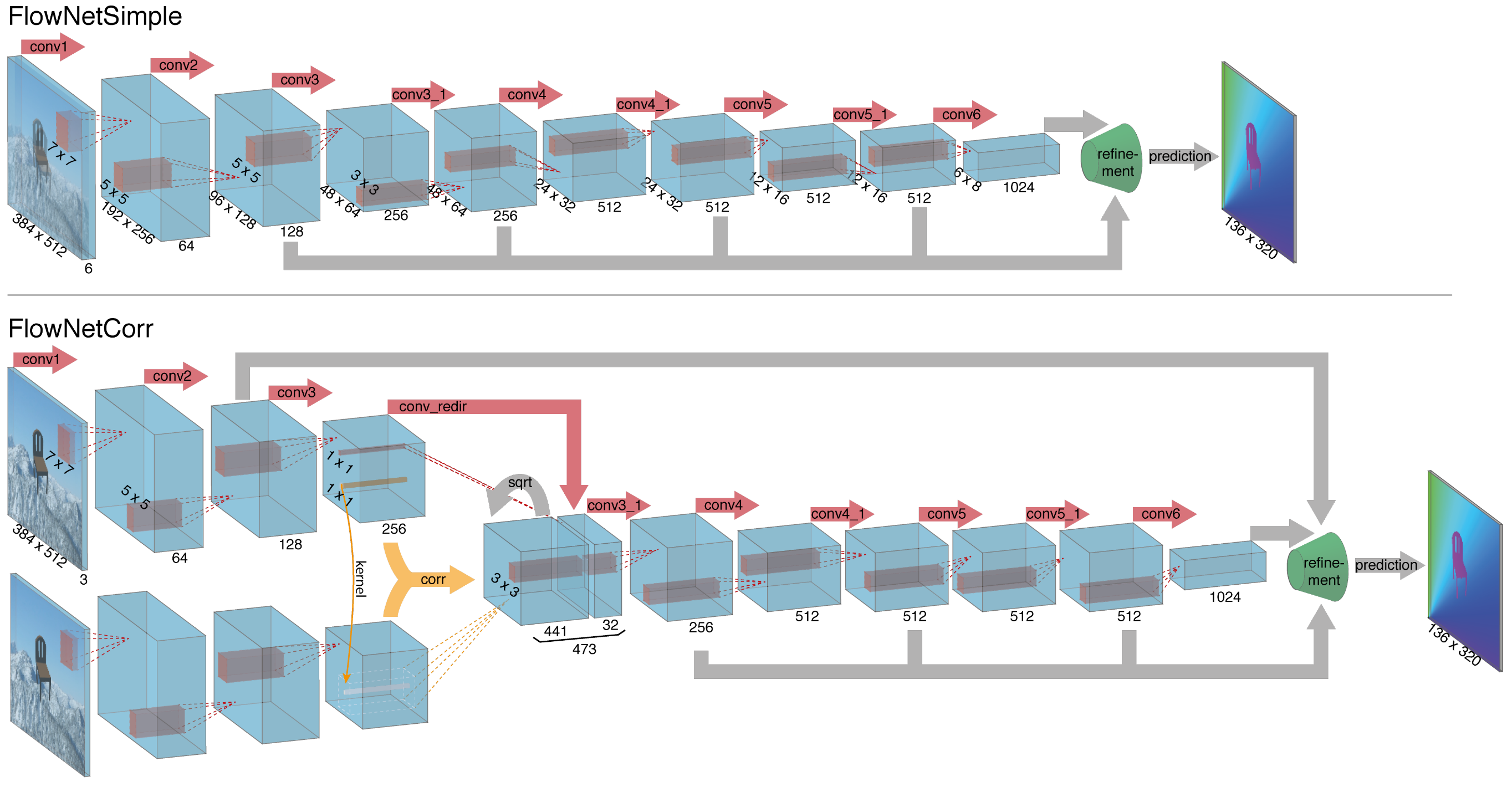
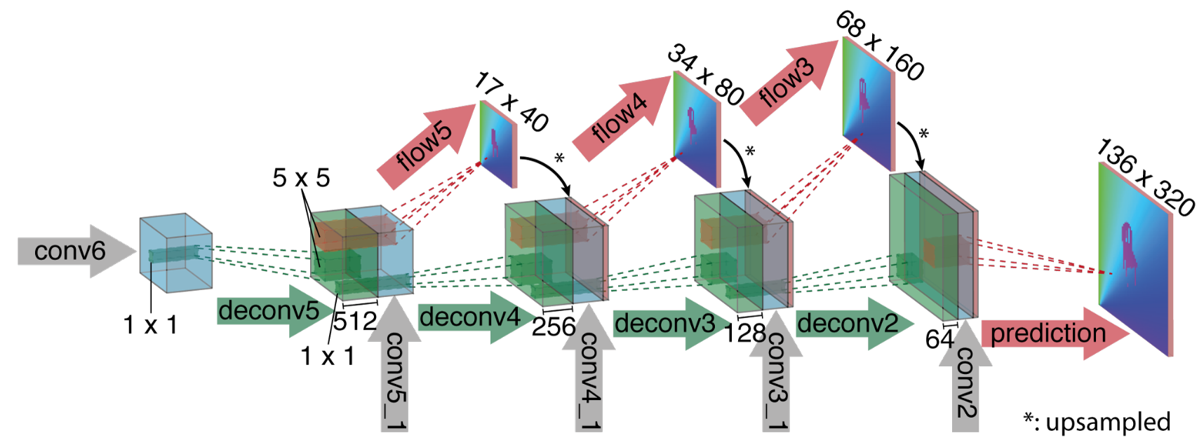
The first end-to-end CNN architecture for estimating optical flow. Two variants:
- FlowNetS
- A pair of input images is simply concatenated and then input to the U-shaped network that directly outputs optical flow.
- FlowNetC
- FlowNetC has a shared encoder for both images, which extracts a feature map for each input image, and a cost volume is constructed by measuring patch-level similarity between the two feature maps with a correlation operation. The result is fed into the subsequent network layers.
Multi-scale training loss is applied. Both models still under-perform energy-based approaches.
FlowNet 2.0 (CVPR 2017) paper
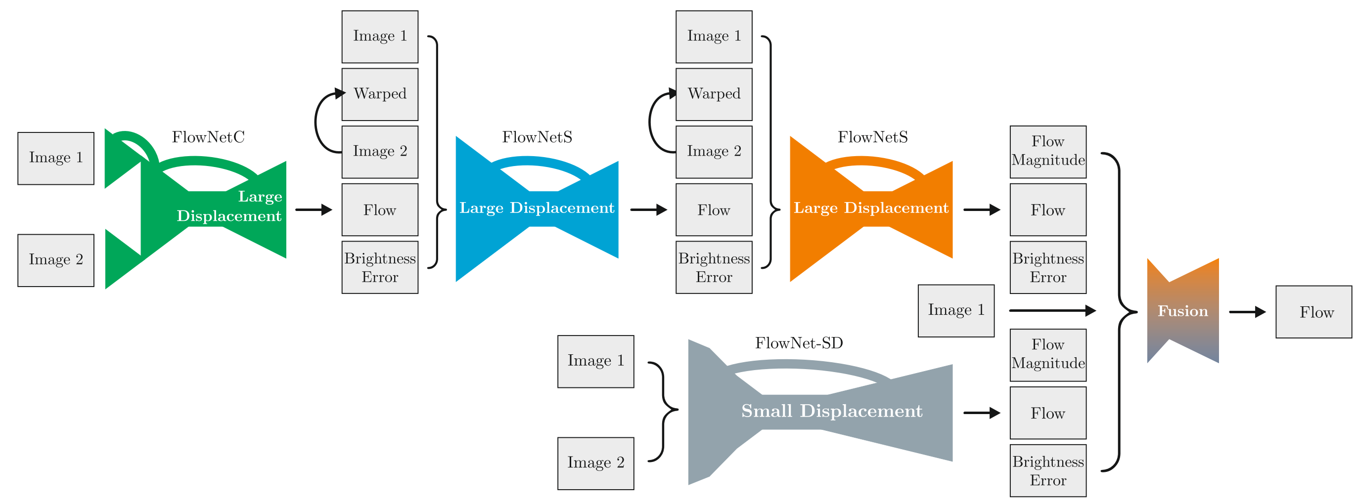
Key ideas:
- By stacking multiple FlowNet style networks, one can sequentially refine the output from previous network modules.
- It is helpful to pre-train networks on a less challenging synthetic dataset first and then further train on a more challenging synthetic dataset with 3D motion and photometric effects
End-to-end based approach starts to outperform energy-based ones.
SPyNet (CVPR 2017) paper code

Key idea:
- Incorporate classic
coarse-to-fineconcepts into CNN network and update residual flow over mulitple pyramid levels (5 image pyramid levels are used). Networks at different levels have separate parameters.
Achieves comparable performance to FlowNet with 96% less number of parameters.
PWCNet (CVPR 2018) paper code video
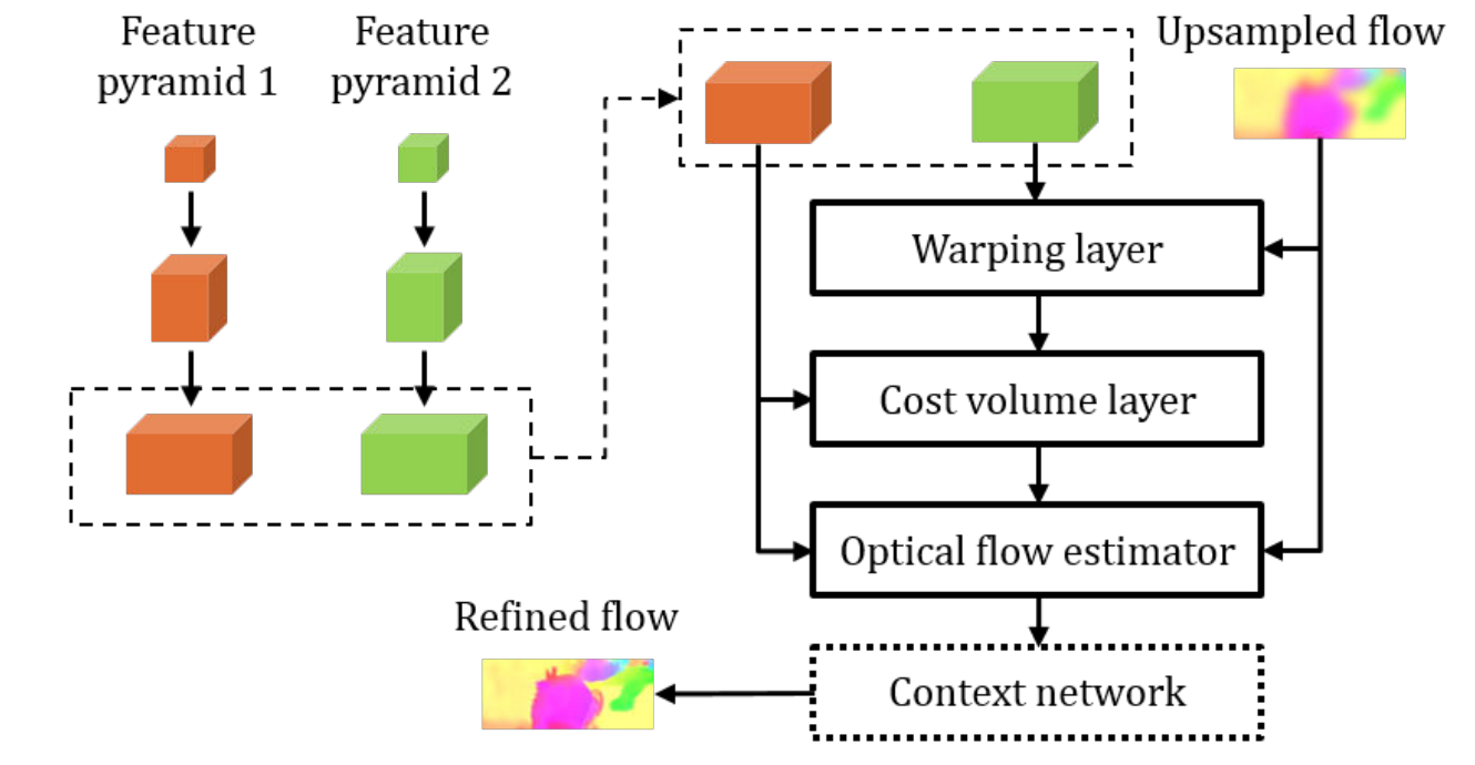
Key ideas:
- Learned feature pyramid instead of image pyramid
- Warping of feature maps
- Computing a cost volume of learned feature maps (correlation)
Computation steps:
- Feature pyramid extractor: conv-net with down-sampling
- Target feature map is warped by up-sampled previous flow estimation
- Cost volume is computed based on source feature map and warped target feature map
- Optical flow estimator: a DenseNet type of network that takes (1) source feature map (2) cost volume (3) up-sampled previous optical flow estimate
- Context network: a dilated convolution network to post process the estimated optical flow
Remarks:
- Multi-scale training loss
- Network at each scale estimates the optical flow for that scale, not the residual optical flow (the addition happens implicitly inside the optical flow estimator).
IRR-PWCNet (CVPR 2019) paper
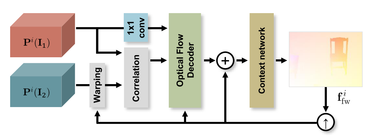
Key ideas
- Take the output from a previous pass through the network as input and iteratively refine it by only using a single network block with shared weights, which allows the network to residually refine the previous estimate.
- For PWCNet, the decoder module at different pyramid level is achieved using a 1x1 convolution before feeding the source feature map to the optical flow estimator/decoder.
- Joint occlusion and bidirectional optical flow estimation leads to further performance enhancement.
PWCNet Fusion (WACV 2019) paper
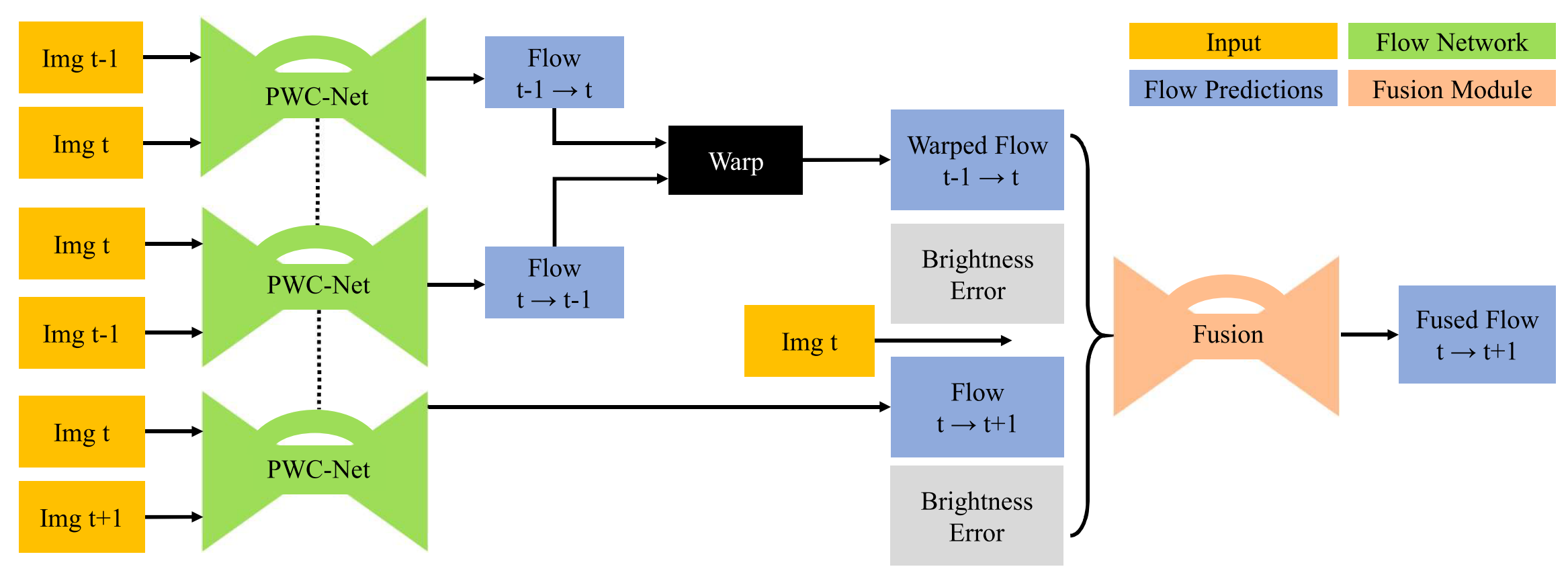
The paper focuses on three-frame optical flow estimation problem: given \(I_{t-1}\), \(I_{t}\), and \(I_{t+1}\), estimate \(f_{t\to t+1}\).
Key ideas:
- If we are given \(f_{t-1\to t}\) and \(f_{t\to t-1}\), and assume constant velocity of movement, then an estimate of \(f_{t\to t+1}\) can be formed by backward warping \(f_{t-1\to t}\) with \(f_{t\to t-1}\). \(\begin{align*} &\widehat{f}_{t\to t+1} \triangleq \texttt{warp}(f_{t-1 \to t}, f_{t\to t-1}), \\ &\widehat{f}_{t\to t+1}(x, y) \triangleq f_{t-1 \to t}\left(x+f_{t\to t-1}(x,y)(x), y+f_{t\to t-1}(x,y)(y)\right) \end{align*}\)
- With three frames available, we can plug-in any two-frame optical flow estimation solution (PWCNet in this case) to obtain \(f_{t-1 \to t}\), \(f_{t\to t+1}\) and \(f_{t \to t-1}\).
- A fusion network (similar to the one used in the last stage of FlowNet 2.0) can be used to fuse together \(\widehat{f}_{t \to t-1}\triangleq\texttt{warp}(f_{t-1 \to t}, f_{t\to t-1})\) and \(f_{t \to t+1}\).
- Note that \(\widehat{f}_{t\to t-1}\) would be identical to \(f_{t\to t+1}\) if (a) velocity is constant (b) three optical flow estimations are correct, and (c) there are no occlusions. Brightness constancy errors of the two flow maps together with the source frame \(I_t\) are fed into the fusion network to provide additional info.
Why multi-frame may perform better than 2-frame solutions:
- temporal smoothness leads to additional regularization.
- longer time sequences may help in ambiguous situations such as occluded regions.
ScopeFlow (CVPR 2020) paper code
ScopeFlow revisits the following two parts in the conventional end-to-end training pipeline/protocol
- Data augmentation:
- photometric transformations: input image perturbation, such as color and gamma corrections.
- geometric augmentations: global or relative affine transformation, followed by random horizontal and vertical flipping.
- cropping
- Regularization
- weighted decay
- adding random Gaussian noises
and advocates
- use larger scopes (crops and zoom-out) when possible.
- gradually reduce regularization
MaskFlownet (CVPR 2020) paper code
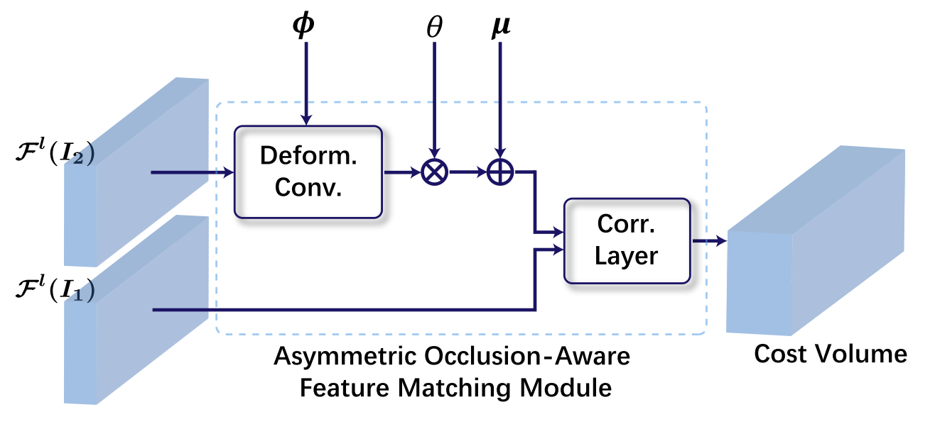
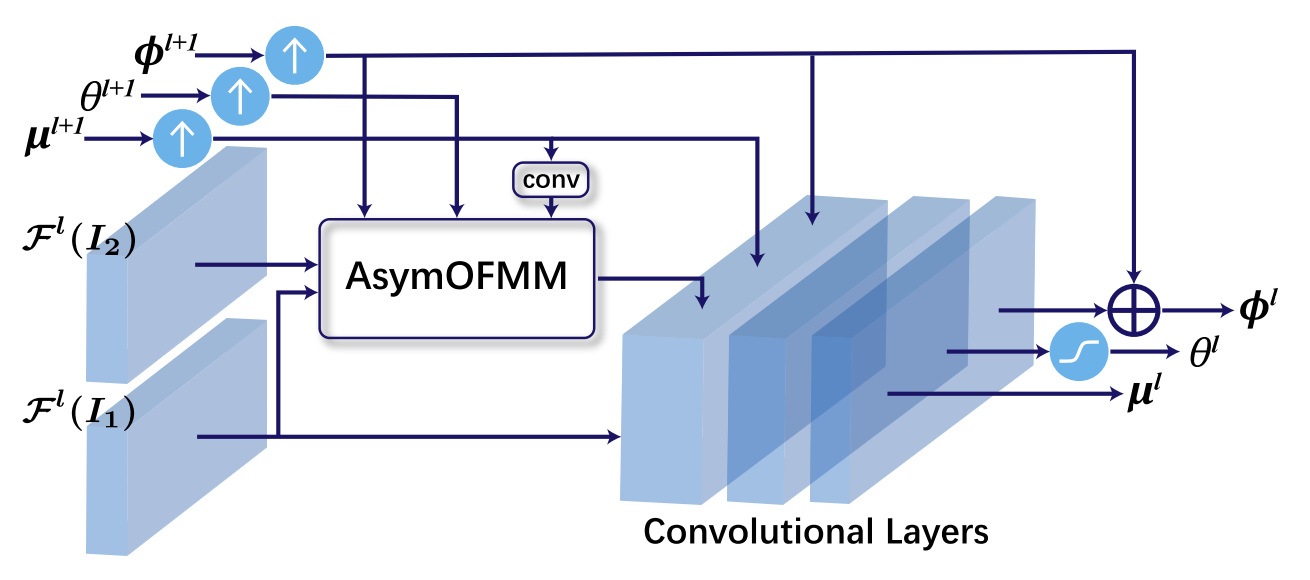
Key idea:
- Incorporates a learnable occlusion mask that filters occluded areas immediately after feature warping without any explicit supervision.