Normalizing Flow: understanding the change of variable equation
Normalizing flow is a technique for constructing complex probability distributions through invertible transformations of a simple distribution. It has been studied and applied in generative models under two contexts: (1) characterizing the approximation posterior distribution of latent variables in the case of variational inference (2) directly approximating the data distribution. When used in the second context, it has demonstrated its capability in generating high-fidelity audio, image, and video data.
The study of generative models is all about learning a distribution \(\mathbb{P}_{\mathcal{X}}\) that fits the data \(\mathcal{X}\) well. With such distribution \(\mathbb{P}(\mathcal{X})\) we can, among other things, generate, by sampling from \(\mathbb{P}_{\mathcal{X}}\), artificial data point that resembles \(\mathcal{X}\). Since the true data distribution lies in high-dimensional space and is potentially very complex, it is essential to have a parameterized distribution family that is flexible and expressive enough to approximate the true data distribution well.
The idea of flow-based methods is to explicitly construct a parameterized family of distributions by transforming a known distribution \(\mathbb{P}_{\mathcal{Z}}\), e.g., a standard multi-variant Gaussian, through a concatenation of function mappings. Let’s consider the elementary case of a single function mapping \(g\). For each sampled value \(z\) from \(\mathbb{P}_{\mathcal{Z}}\), we map it to a new value \(x=g(z)\).
\[\begin{align*} z \xrightarrow{g(.)} x \end{align*}\]Up until this point, we have not introduced anything new. This way of transforming a known distribution using a function mapping \(g\) is also adopted by generative adversarial networks (GAN). The question that flow-based method asks is: can we get a tractable probability density function (pdf) of \(x=g(z)\)? If so, we can directly optimize the probability density of the dataset, i.e., the log likelihood of the data, rather than resorting to the duality approach adopted by GAN, or the lower-bound approach adopted by VAE.
Unfortunately, for a general function \(g\) that maps \(z\) to \(x\), the pdf of the new random variable \(x=g(z)\) is quite complicated and usually intractable due to the need to calculate a multi-dimensional integral. However, if we restrict \(g\) to be a bijective (one-to-one correspondence) and differentiable function, then the general change-of-variable technique reduces to the following tractable form:
\[\begin{align*} \mathbb{P}_\mathcal{X}(x) = \mathbb{P}_{\mathcal{Z}}(z)\left|\det \frac{d g(z)}{d z}\right|^{-1}, x=g(z) \end{align*}\]An important consequence with the bijective assumption is that \(z\) and \(x\) must have the same dimension: if \(z\) is a \(d-\)dimensional vector \(z=[z_1, z_2, \ldots, z_d]\), the corresponding \(x\) must also be a \(d-\)dimensional vector \(x=[x_1, x_2, \ldots, x_d]\). It is worth emphasizing that the bijective assumption is essential to the tractability of the change-of-variable operation, and the resulting dimension invariance is a key restriction in flow-based methods.
The above equation, albeit tractable, looks by no means familiar or friendly — what is with the absolute value? the determinant? the Jacobian? the inverse? The whole equation screams for an intuitive explanation. So here we go — let’s gain some insights into the meaning of the formula.
First off, since \(g\) is bijective and thus invertible, we can denote the inverse of \(g\) as \(f=g^{-1}\), which allows us to rewrite the equation as
\[\begin{align*} \mathbb{P}_\mathcal{X}(x) = \mathbb{P}_{\mathcal{Z}}(f(x))\left|\det \frac{d x}{d f(x)}\right|^{-1} = \mathbb{P}_{\mathcal{Z}}(f(x))\left|\det \frac{d f(x)}{d x}\right| \end{align*}\]In the last equation, we get rid of the inverse by resorting to the identity that the determinant of an inverse is the inverse of the determinant, the intuition of which will become clear later.
To understand the above equation, we start with a fundamental invariance in the change of probability random variables: the probability mass of the random variable \(z\) in any subset of \(\mathcal{Z}\) must be the same as the probability mass of \(x\) in the corresponding subset of \(\mathcal{X}\) induced by transformation from \(z\) to \(x\), and vice versa.
Let us exemplify the above statement with an example. Consider the case when \(x\) and \(z\) are 2 dimensional, and focus on a small rectangular in \(\mathcal{X}\) defined by two corner points \((a, b)\) and \((a+\Delta x_1, b + \Delta x_2)\). If \(\Delta x_1\) and \(\Delta x_2\) are small enough, we can approximate the probability mass on the rectangular as the density \(\mathbb{P}_\mathcal{X}\) evaluated at point \((a,b)\) times the area of the rectangular. More precisely,
\[\begin{align*} &P {\big(} (x_1, x_2) \in [a, a+\Delta x_1]\times[b, b+\Delta x_2] {\big)}\\ \approx& \mathbb{P}_\mathcal{X} ((a, b)) \times \text{area of }[a, a+\Delta x_1]\times[b, b+\Delta x_2]\\ =&\mathbb{P}_\mathcal{X} ((a, b)) \Delta x_1 \Delta x_2 \end{align*}\]This approximation is basically assuming that the probabilistic density on the rectangular stays constant and equal to \(\mathbb{P}_\mathcal{X} ((a, b))\), which holds asymptotically true as we shrink the width \(\Delta x_1\) and height \(\Delta x_2\) of the rectangular. The left figure below provides an illustration.
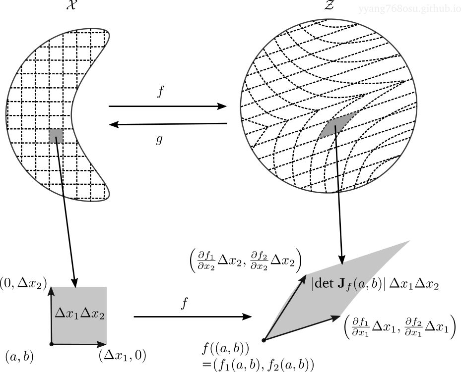
Now resorting to the aforementioned invariance, the probability mass on the \(\Delta x_1 \times \Delta x_2\) rectangular must remain unchanged after the transformation. So what does the rectangular look like after the transformation of \(f\)? Let us focus on the corner point \((a+\Delta x_1, b)\):
\[\begin{align*} f((a+\Delta x_1, b))=&(f_1(a+\Delta x_1,b), f_2(a+\Delta x_1,b)) \\ =& (f_1(a,b), f_2(a,b)) \\ +& \left(\frac{\partial f_1}{\partial x_1}(a, b)\Delta x_1 , \frac{\partial f_2}{\partial x_1}(a, b)\Delta x_1\right) \text{ }\text{ first order component} \\ +& \left(o(\Delta x_1), o(\Delta x_1)\right) \text{ }\text{ second and higher order residual} \end{align*}\]With \(\Delta x_1\) and \(\Delta x_2\) small enough, we can just ignore the higher order term and keep the linearized term. As can be seen from the figure above, the rectangular area is morphed into a parallelogram defined by the two vectors
\[\begin{align*} &\left(\frac{\partial f_1}{\partial x_1}(a, b)\Delta x_1 , \frac{\partial f_2}{\partial x_1}(a, b)\Delta x_1\right)\\ &\left(\frac{\partial f_1}{\partial x_2}(a, b)\Delta x_2 , \frac{\partial f_2}{\partial x_1}(a, b)\Delta x_2\right) \end{align*}\]We have geometry to tell us that the area of a parallelogram is just the absolute determinant of the matrix composed of the edge vectors, which is expressed as below.
\[\begin{align*} {\Bigg|} \det \underbrace{\left[ \begin{array}{ll} \frac{\partial f_1}{\partial x_1} & \frac{\partial f_2}{\partial x_1}\\ \frac{\partial f_1}{\partial x_2} & \frac{\partial f_2}{\partial x_2} \end{array} \right]_{(a,b)}}_{\substack{\text{Jacobian of $f$}\\\text{evaluated at $(a,b)$}}} {\Bigg |} \Delta x_1 \Delta x_2 \end{align*}\]By plugging in the above into the invariance statement, we reached the following identity
\[\begin{align*} \mathbb{P}_\mathcal{X} ((a, b)) \Delta x_1 \Delta x_2 = \mathbb{P}_\mathcal{Z} (f(a, b)) \left|\det {\bf J}_f(a,b)\right| \Delta x_1 \Delta x_2 \end{align*}\]With \(\Delta x_1\Delta x_2\) canceled out, we reached our target equation
\[\begin{align*} \mathbb{P}_\mathcal{X} (x) = \mathbb{P}_\mathcal{Z} (f(x)) \left|\det {\bf J}_f(x)\right| = \mathbb{P}_\mathcal{Z} (f(x)) \left|\det \frac{\partial f(x)}{\partial x}\right|. \end{align*}\]For data with dimension larger than two, the above equation still holds, with the distinctions that the parallelogram becomes a parallelepiped, and the concept of area becomes a more general notion of volume.
It should be clear now what the physical interpretation is for the absolute-determinant-of-Jacobian — it represents the local, linearized rate of volume change (quoted from this excellent blog) for the function transform. Why do we care about the rate of volume change? exactly because of the invariance of probability measure — in order to make sure each volume holds the same measure of probability before and after the transformation, we need to factor in the volume change induced by the transformation.
With this interpretation that the absolute-determinant-of-Jacobian is just local linearized rate of volume change, it should not be surprising that the determinant of a Jacobian of an inverse function is the inverse of the determinant Jacobian of the original function. In other words, if function \(f\) expands a volume around \(x\) by rate of \(r\), then the inverse function \(g=f^{-1}\) must shrink a volume around \(f(x)\) by the same rate of \(r\).