A step-by-step guide to variational inference (4): variational auto encoder
The variational lower bound \(\mathcal{L}\) sits in the core of variational inference. It connects the density estimation problem with the Bayesian inference problem through a variational (free to vary) distribution \(q\), and it converts both problems into an optimization problem. Here let’s briefly revisit the identity associated with variational lower bound
\[\begin{align*} \ln p(X;\theta) &= \text{KL}{\big(}q|| p(Z|X;\theta){\big)} + \mathcal{L}(q,\theta)\\ \text{where }\mathcal{L}(q, \theta) &=\int q(Z) \ln \frac{p(X,Z;\theta)}{q(Z)} dZ \end{align*}\]The identity holds for any arbitrary probability function \(q\). \(\mathcal{L}\) is a lower bound for the data log-likelihood \(\ln p(X;\theta)\) given the non-negativity of the KL divergence. From the identify we can obtain the following two equations
\[\begin{aligned} \ln p(X;\theta) &= \max_{q} \mathcal{L}(q,\theta)\\ p(Z|X;\theta) &= \underset{q}{\arg\max} \mathcal{L}(q,\theta), \end{aligned}\]which testifies the claim that both density estimation (LHS of the first equation) and Bayesian inference (LHS of the second equation) are linked with the same optimization function. There are two implications if we increases the value of \(\mathcal{L}\) by tweaking the distribution \(q\): (1) \(\mathcal{L}\) becomes a tighter lower bound of \(\ln p(X;\theta)\), meaning that it is closer to the true data log-likelihood in value (2) the distribution function \(q\) itself is closer to the true posterior distribution measured in KL divergence.
Often, we are also given the task of finding the ML estimate of the parameter \(\theta\) (or MAP estimate of the parameter \(\theta\)), which requires taking the maximum of \(\ln p(X;\theta)\) (or \(\ln p(X\|\theta) + \ln p_\text{prior}(\theta)\) for the MAP case) with respect to \(\theta\), yielding the following problem
\[\begin{align*} \max_{\theta}\max_{q}\mathcal{L}(q, \theta). \end{align*}\]By increasing the variational lower bound \(\mathcal{L}\) with respect to \(\theta\), by which the model is parameterized, we are essentially searching for model that can better fit to the data.
It should be clear that is it desirable to maximize \(\mathcal{L}\) with respect to both the variational distribution \(q\) and the generative parameter \(\theta\): maximize it with respect to \(q\) would yield a better inference function; maximize it with respect to \(\theta\) would give us a better model.
Instead of allowing \(q\) to be any function within the probability function space, for analytical tractability, we assume that it is parameterized by \(\phi\) and is a function of the observed data \(x\), denoted as \(q_\phi(x)\). For the generative model, let us modified the notation slightly by assuming that the prior distribution \(p(z)\) is unparameterized, and denote the conditional generative probability as \(p_\theta(x\|z)\), leading to the following expression of the variational lower bound
\[\begin{align*} \mathcal{L}(\phi, \theta, x^{(i)}) = \int q_\phi\left(z^{(i)}|x^{(i)}\right)\ln \frac{p_\theta\left(x^{(i)}|z^{(i)}\right)p\left(z^{(i)}\right)}{q_\phi\left(z^{(i)}|x^{(i)}\right)}dz^{(i)} \end{align*}\]Note that we used to express the variational lower bound in terms of the complete observed dataset \(X=\{x^{(1)},\ldots, x^{(N)}\}\) as well as the corresponding latent variables \(Z=\{z^{(1)},\ldots, z^{(N)}\}\). Since each data point and the corresponding latent variables are generated independently, it can be decomposed into the summation of \(N\) terms, one for each data point \(x^{(i)}\) as shown above. Those \(N\) identity equations are linked through global parameter \(\phi\) and \(\theta\).
As discussed before, to obtain a better model and to obtain a closer approximation to the true posterior inference function, one needs to differentiate and optimize \(\sum_{i=1}^N\mathcal{L}(\phi, \theta, x^{(i)})\) with respect to both \(\phi\), the parameter of the inference function, and \(\theta\), the parameter of the model. Here’s a plan: let us calculate the gradient for the lower bound with respect to both parameters, and be done with the problem by applying our favorite stochastic gradient descent algorithm to find a solution. Actually we will show later that such a stochastic training framework is analogous to using an auto-encoder architecture with a specific regularization function.
A major challenge arises: it is not clear how to differentiate against \(\phi\). There is very little chance of obtaining a closed-form expression by directly differentiating inside the integral, as the integral itself is hard even without the differentiation. We now examine this issue carefully, as it is the key to understanding the variational auto-encoding algorithm.
Since the lower-bound exists in the form of the expectation with respect to the variational distribution \(q_\phi\), the work-around here is to seek for Monte-Carlo estimation for the integral with the sampling from distribution \(q_\phi\left(z^{(i)}\|x^{(i)}\right)\). Let us focus on the general problem of \(\nabla_\phi \mathbb{E}\_{q_\phi(z\|x)}\left[f(z)\right]\), for which there are two approaches that use sampling to approximate the expectation:
Approach 1:
\[\begin{align*} &\nabla_\phi \mathbb{E}_{q_\phi(z|x)}\left[f(z)\right] \\ =&\int \nabla_\phi q_\phi(z|x) f(z) dz\\ =&\int q_\phi(z|x) \frac{\nabla_\phi q_\phi(z|x)}{q_\phi(z|x)} f(z) dz\\ =& \int q_\phi(z|x) \nabla_\phi \ln q_\phi(z|x) f(z) dz \\ =& \mathbb{E}_{q_\phi(z|x)}\left[ \nabla_\phi \ln q_\phi(z|x) f(z)\right] \\ \text{(Monte Carlo)} \approx &\frac{1}{S}\sum_{s=1}^S \nabla_\phi \ln q_\phi(z^{[s]}|x) f(z^{[s]}) \end{align*}\]Approach 2:
This approach makes an additional assumption on \(q_\phi(z\|x)\): assume that we can obtain samples of \(z\) by first sampling through a distribution \(p(\epsilon)\) that is independent of \(\phi\), and then apply a \((\phi,x)\)-dependent transformation of \(g_\phi(\epsilon, x)\). Effectively we are assuming that the random variable \(\mathcal{Z}\) is a \(\phi-\)dependent function of a \(\phi\)-independent random variable \(\mathcal{E}\): \(\mathcal{Z} = g_\phi(\mathcal{E},x)\). Reflecting this assumption in the differential of expectation, we obtain
\[\begin{align*} &\nabla_\phi \mathbb{E}_{q_\phi(z|x)}\left[f(z)\right]\\ =&\nabla_\phi \int q_\phi(z|x)f(z) dz\\ \text{(parameter substitution)}=&\nabla_\phi \int p(\epsilon)f(g_\phi(\epsilon, x))d\epsilon\\ =& \int p(\epsilon) \nabla_\phi f(g_\phi(\epsilon, x))d\epsilon\\ \text{(Monte Carlo)}\approx& \frac{1}{S}\sum_{s=1}^S \nabla_\phi f(g_\phi(\epsilon^{[s]},x)) \end{align*}\]This seems like a good solution: the Monte Carlo sampling itself is not a function of \(\phi\), and \(\phi\) just appear as the parameter of the transformation function \(g_\phi\) that maps the samples from \(\mathcal{E}\) to the samples in \(\mathcal{Z}\). In this case \(q_\phi\) is just the induced distribution as a function of the prior distribution of \(\mathcal{E}\) as well as the transformation function \(g_\phi\). This parameter substitution technique is branded as the reparameterization trick in the original paper of variational auto encoder.
To understand the implication of such assumption, let’s ask this question: is it feasible to design the prior distribution of \(\mathcal{E}\) and the transformation function \(g_\phi\) in any arbitrary form? You may wonder why do we even care. Well there is a hidden factor that we need to take care of before claiming victory. Looking at the variational lower bound expression, not only do we need to integrate with respect to the distribution \(q_\phi\), which can be achieved using Monte Carlo by the help of this reparameterization trick, we also need to ensure a closed-form expression of the density function \(q_\phi(z\|x)\) itself, as it lives inside the expectation/integral. This limits the way we can choose the random variable \(\mathcal{E}\) and the function \(g_\phi\).
To investigate on the requirement of \(\mathcal{E}\) and \(g_\phi\) such that the induced random variable \(\mathcal{Z} = g_\phi(\mathcal{E},x)\) has a tractable density/distribution function (easy to evaluate), let’s try to express distribution \(q_\phi\) as a function of \(p_\epsilon\) and \(g_\phi(z,x)\). For any monotonic function \(g_\phi\), the induced distribution \(q_\phi\) can be derived as
\[\begin{align*} q_\phi(z) = p_\epsilon\left(g_\phi^{-1}(z)\right)\left|\frac{\partial g_\phi^{-1}(z)}{\partial z}\right|. \end{align*}\]To enforce a closed form expression for \(q_\phi\), we have two general design choices on \(p_\epsilon\) and \(g_\phi\), as is evident from the expression above: (1) let \(p_\epsilon\) be a uniform distribution on \([0,1]\) and \(g_\phi=\text{CDF}^{-1}\) be the inverse of any distribution with closed-form cumulative distribution function. (2) let \(p_\epsilon\) be any distribution with closed form density and \(g_\phi\) be an easy form of monotonic function, e.g., a linear function.
In the context of variational auto encoder in the original paper, the second design choice is picked: \(p_\epsilon\) is chosen as the standard normal distribution and \(g_\phi\) is a linear function of \(\epsilon\), whose slope and intercept is an arbitrary function of \(x\) and \(\phi\) characterized using a neural network. In this case the induced distribution \(q_\phi\) is a normal distribution whose mean and variances is determined by a neural network with the input \(x\) and parameter \(\phi\).
Now that we went through what the reparameterization trick is, let us return to the problem of finding the gradient of \(\mathcal{L}(\phi, \theta, x^{(i)})\) with respect to \(\phi\) and \(\theta\). Applying the reparameterization trick, we obtain the following gradient-friendly Monte Carlo estimate of the variational lower bound
\[\begin{align*} \mathcal{L}(\phi, \theta, x^{(i)}) =& \int q_\phi\left(z^{(i)}|x^{(i)}\right)\ln \frac{p_\theta\left(x^{(i)}|z^{(i)}\right)p\left(z^{(i)}\right)}{q_\phi\left(z^{(i)}|x^{(i)}\right)}dz^{(i)}\\ \text{(Monte Carlo)}\approx&\frac{1}{S}\sum_{s=1}^S \ln \frac{p_\theta\left(x^{(i)}|z^{(i)[s]}\right)p\left(z^{(i)[s]}\right)}{q_\phi\left(z^{(i)[s]}|x^{(i)}\right)}\\ \text{(Reparameterization)}=&\frac{1}{S}\sum_{s=1}^S \ln \frac{p_\theta\left(x^{(i)}|g_\phi (\epsilon^{[s]}, x^{(i)})\right)p\left(g_\phi (\epsilon^{[s]}, x^{(i)})\right)}{q_\phi\left(g_\phi (\epsilon^{[s]}, x^{(i)})|x^{(i)}\right)}\\ \text{where } \epsilon^{[s]}&\text{ is drawn i.i.d. from }p_\epsilon. \end{align*}\]Here’s an alternative way to decompose \(\mathcal{L}\) and apply Monte Carlo and reparameterization, for which there is a close form expression for the second term (KL divergence) and only the first part is approximated.
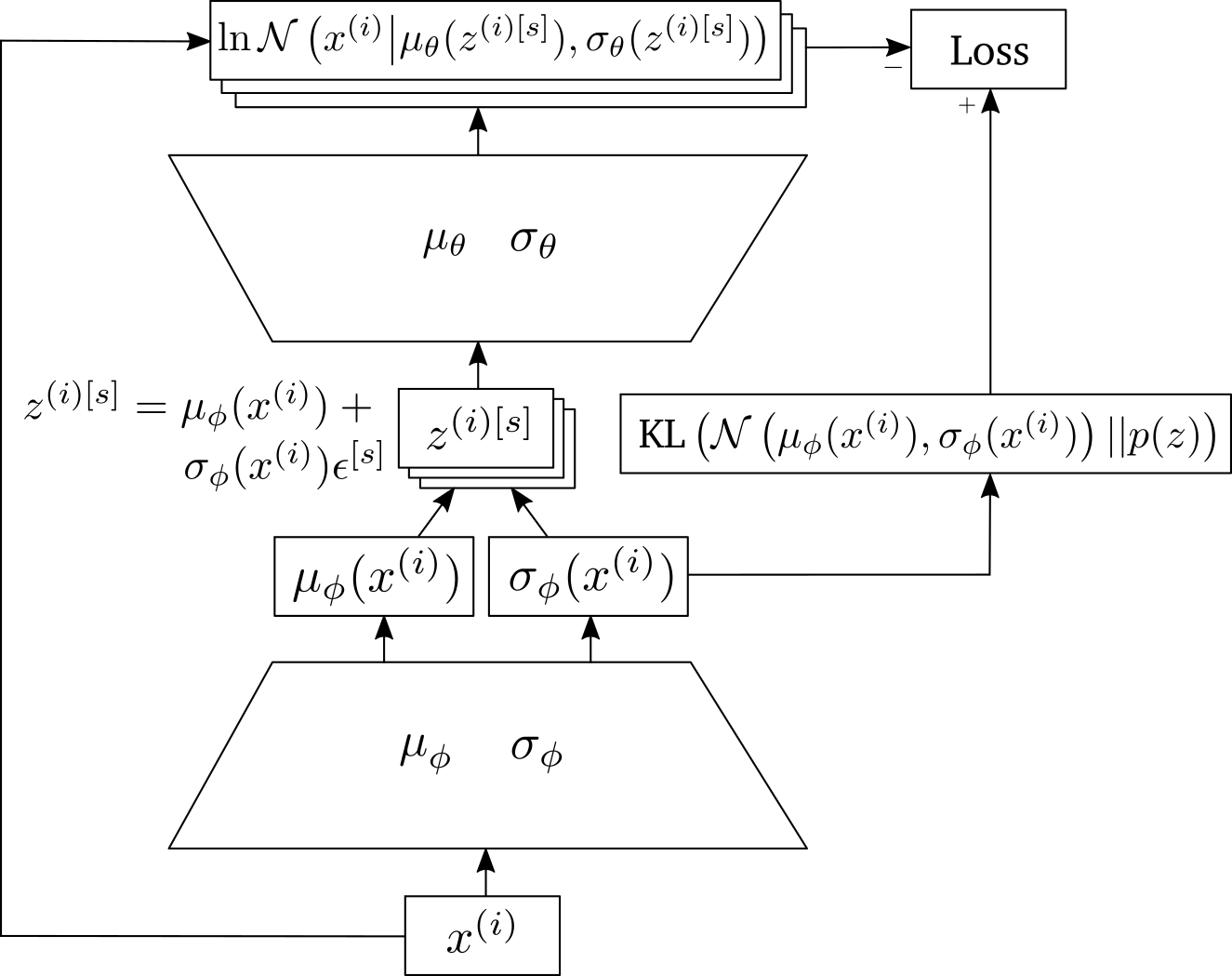
\[\begin{align*} \mathcal{L}(\phi, \theta, x^{(i)}) =& \int q_\phi\left(z^{(i)}|x^{(i)}\right)\ln \frac{p_\theta\left(x^{(i)}|z^{(i)}\right)p\left(z^{(i)}\right)}{q_\phi\left(z^{(i)}|x^{(i)}\right)}dz^{(i)}\\ =&\int q_\phi\left(z^{(i)}|x^{(i)}\right)\ln p_\theta\left(x^{(i)}|z^{(i)}\right) dz^{(i)}-\text{KL}\left( q_\phi\left(z^{(i)}|x^{(i)}\right){\Big|\Big|} p\left(z^{(i)}\right)\right)\\ \text{(Monte Carlo)}\approx& \frac{1}{S}\sum_{s=1}^S \ln p_\theta\left(x^{(i)}|z^{(i)[s]}\right) -\text{KL}\left( q_\phi\left(z^{(i)}|x^{(i)}\right){\Big|\Big|} p\left(z^{(i)}\right)\right)\\ \text{(Reparameterization)}\approx& \frac{1}{S}\sum_{s=1}^S \ln p_\theta\left(x^{(i)}|g_\phi (\epsilon^{[s]}, x^{(i)})\right) -\text{KL}\left( q_\phi\left(z^{(i)}|x^{(i)}\right){\Big|\Big|} p\left(z^{(i)}\right)\right) \end{align*}\]This decomposition leads to the interpretation of probabilistic auto-encoder, which is named variational auto-encoder as it rooted from the maximization of the variational lower bound.